The description of the Excel program is the most important. Microsoft Excel: brief information about the program.

Microsoft Excel the program is designed to organize data in a table for documentation and graphical representation information. MS Excel workbooks provide the ability to store and organize data for calculating the sum of values ​​in cells...

Share your work on social networks

If this work does not suit you, at the bottom of the page there is a list of similar works. You can also use the search button

CONTENT

I Introduction II Main part 2.1 Description of MS Excel program functions 1.2 Program window 1.4Spreadsheet structure 1.5. Functions 1. 6 Possible mistakes when using functions in formulas 1.7 Data types and analysis 1.7 Scenarios III Practical part 3.1 Application of functions 3.2. Applying a script 3.2.1. Example of calculations of the internal investment turnover rate 3.2. Building charts IV. Workplace organization V. Occupational safety while working with a PC VI. Bibliography

I Introduction

Microsoft Excel is a program designed to organize data in a table for documenting and graphically presenting information.

MS Excel is used to create complex documents that require:

· Use the same data in different worksheets;

· Change and restore connections.

The advantage of MS Excel is that the program helps to operate with large volumes of information. MS Excel workbooks provide the ability to store and organize data and calculate the sum of values ​​in cells. MS Excel provides a wide range of methods to make information easy to understand.

Nowadays, it is important for every person to know and have skills in working with applications Microsoft Office, because modern world saturated a huge amount information that you simply need to be able to work with.

Goal: get acquainted with the functions of MS Excel for data processing

Task: consider the practical application of functions MS Excel

II Main part

2.1 Description of MS Excel program functions

1.2 Program window

To launch Excel, run Start / Programs / Microsoft Office / Microsoft Excel.

After downloading the program it will open working window Microsoft Excel, which contains menu items, as well as toolbars that contain buttons for creating a new workbook, opening an existing one, etc.

Window Microsoft programs Excel with the loaded spreadsheet will look like the one shown in Figure 1.

Figure 1. - Microsoft Excel program window

The main elements of the working window are:

1. Title bar (it indicates the name of the program) with buttons for controlling the program window and document window (Collapse, Minimize to window or Expand to full screen, Close);

2. Main menu bar (each menu item is a set of commands united by a common functional focus) plus a window for searching for help information.

3. Toolbars ( Standard Formatting and etc.).

4. The formula bar, containing the Name field and the Insert Function (fx) button as elements, is intended for entering and editing values ​​or formulas in cells. The Name field displays the address of the current cell.

5. Workspace(active worksheet).

6. Scroll bars (vertical and horizontal).

7. A set of shortcuts (sheet shortcuts) for moving between worksheets.

8. Status bar

1.4Spreadsheet structure

A file created using MS Excel is commonly called a workbook. You can create as many workbooks as your availability allows. free memory on the appropriate memory hardware. You can open as many workbooks as you have created. However, only one current (open) workbook can be an active workbook.

A workbook is a collection of worksheets, each of which has a tabular structure. The document window displays only the current (active) worksheet with which you are working. Each worksheet has a title, which appears on the worksheet tab at the bottom of the window. Using shortcuts, you can switch to other worksheets included in the same workbook. To rename a worksheet, you need to double-click on its tab and replace the old name with a new one or by executing following commands: Format menu, Sheet line in the Rename menu list. Or you can, by placing the mouse pointer on the active worksheet shortcut, right-click, then in the context menu that appears, click on the Rename line and perform a rename. You can add (insert) new sheets to the workbook or delete unnecessary ones. Inserting a sheet can be done by executing the Insert menu command, line Sheet in the list of menu items. The sheet will be inserted before the active sheet. The above steps can also be accomplished using context menu, which is activated by pressing right button mouse, the pointer of which should be placed on the tab of the corresponding sheet. To swap worksheets, you need to place the mouse pointer on the tab of the sheet being moved, click left button mouse and drag the shortcut to the desired location.

A worksheet (table) consists of rows and columns. Columns are headed in capitals with Latin letters and, further, two-letter combinations. The worksheet contains a total of 256 columns, named A through IV. The lines are numbered sequentially from 1 to 65536.

Table cells are formed at the intersection of columns and rows. They are the minimum elements designed to store data. Each cell has its own address. A cell address consists of the column name and row number at the intersection of which the cell is located, for example, A1, B5, DE324. Cell addresses are used when writing formulas that define the relationship between values ​​located in different cells. Data entry and editing operations are always carried out only in the active cell. Data located in adjacent cells that form a rectangular area can be referenced as a single unit in formulas. A group of cells bounded by a rectangular area is called a range. The most commonly used rectangular ranges are formed at the intersection of a group of sequential rows and a group of sequential columns. A range of cells is indicated by indicating the address of the first cell and the address of the last cell in the range, separated by a colon, for example, B5: F15. Selecting a range of cells can be done by dragging the mouse pointer from one corner cell to the opposite cell diagonally. The frame of the current (active) cell expands, covering the entire selected range. Fig.2

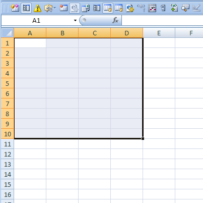
Fig.2

To speed up and simplify computational work Excel puts at the user's disposal a powerful apparatus of worksheet functions that allow almost all possible calculations to be carried out.

1.5. Functions

In total, MS Excel contains more than 400 worksheet functions (built-in functions). All of them, according to their purpose, are divided into 11 groups (categories):

1. financial functions;

2. date and time functions;

3. arithmetic and trigonometric (mathematical) functions;

4. statistical functions;

5. functions of links and substitutions;

6. database functions (list analysis);

7. text functions;

8. logical functions;

9. information functions(checking properties and values);

10.function engineering;

11. Higher functions.

Writing any function into a worksheet cell must begin with the equals symbol (=). If the function is used as part of any other complex function or in a formula (mega formula), then the symbol exactly (=) is written before this function (formula). Any function is accessed by specifying its name followed by an argument (parameter) or list in parentheses. Availability parentheses necessarily, they serve as a sign that the name used is the name of a function. List parameters (function arguments) are separated by semicolons (;). Their number should not exceed 30, and the length of a formula containing as many calls to functions as desired should not exceed 1024 characters. When writing (entering) a formula, it is recommended to type all names lowercase letters, then correctly entered names are displayed in capital letters.

1. 6 Possible errors when using functions in formulas

When working with spreadsheets, it is important not only to know how to use them, but also to avoid making common mistakes. Research has shown that more than half of people who frequently use Microsoft Excel in their work keep it on their desktop regular calculator! The reason turned out to be simple: to perform the operation of summing two or more cells to obtain intermediate result(and, as practice shows, most people have to perform such an operation quite often), it is necessary to perform two extra steps. Find the place in the current table where it will be located total amount, and activate the summation operation by pressing the S (sum) button. And only after that you can select those cells whose values ​​are supposed to be summed.

In an Excel cell, you may see ####### (sharp) instead of the expected calculated value. This is just a sign that the cell width is not sufficient to display the resulting number.

The following values, called error constants, Excel displays in cells as formulas containing if errors occur in the calculations of these formulas:

1. # NAME? - The function name or cell address was entered incorrectly.

2. #DIV / 0! - The value of the denominator in the formula equal to zero(division by zero).

3. #NUMBER! - The function argument value is not valid. For example, ln(0), ln(-2),.

4. # VALUE! - The function parameters were entered incorrectly. For example, instead of a range of cells, their sequential listing was introduced.

1.6 Data analysis in MS Excel

Data - information:

Obtained by measurement, observation, logical or arithmetic operations;

Presented in a form suitable for permanent storage, transmission and (automated) processing.

1.7 Data types and analysis

IN Excel type data - type, value stored in the cell.

When data is entered into a worksheet, Excel automatically analyzes it to determine the data type. The default data type assigned to a cell determines the data analysis that can be applied to that cell.

For example, most data analysis tools use numeric values. If you try to enter text meaning, the program will respond with an error message.

Data types:

1. Text

2. Numeric

3. Number

4. Numeric characters

5. Fractions

6. Date and time

7. Give

8. Time

9. Formulas

Data analysis is a field of computer science that deals with the construction and study of the most common mathematical methods and computational algorithms for extracting knowledge from experimental (in in a broad sense) data.

Data analysis - comparison of various information.

Working with a table is not limited to simply entering data into it. It is difficult to imagine an area where analysis of this data would not be required.

Data tables are part of a block of tasks that are sometimes called what-if analysis tools. The data table is a range of cells showing how the change certain values in formulas affects the results of those formulas. Tables provide a way to quickly calculate multiple versions within a single operation, as well as a way to view and compare the results of all various options on one sheet.

MS Excel presents ample opportunities to analyze the data in the list. Analysis tools include:

Processing a list using various formulas and functions;

Constructing charts and using MS Excel maps;

Checking data from worksheets and workbooks for errors;

Structuring worksheets;

Automatic summarization (including partial sum wizard);

Data consolidation;

Pivot tables;

Special means analysis of sample records and data - selection of parameters, search for solutions, scenarios, etc.

1.7 Scenarios

One of the main benefits of data analytics is predicting future events based on today's information.

Scripts are part of a block of tasks that are sometimes called what-if analysis tools. (What-if analysis: The process of changing cell values ​​and analyzing the effect THOSE changes have on the result of formula calculations on a worksheet, such as changing the interest rate used in a depreciation table to determine payment amounts.)

A script is a set of values ​​that are Microsoft application Office Excel are saved and can be automatically inserted into the sheet. Scenarios can be used to predict the results of worksheet calculation models. It is possible to create and save different groups of values ​​in a worksheet, and then switch to any of these new scenarios to view different results. Or you can create multiple input datasets ( changeable cells) for any number of variables and assign a name to each set. Based on the name of the selected data set, MS Excel will generate the analysis results on the worksheet. In addition, the scenario manager allows you to create a final report on scenarios, which reflects the results of the substitution various combinations input parameters.

As you develop the scenario, the data on the sheet will change. For this reason, before starting to work with the script, you will need to create a script that saves the original data, or create a copy of the Excel sheet.

All scripts are created in the Add Script dialog box. First, you need to specify the cells to display the predicted changes. Cell references are separated from each other by a colon or semicolon. The Scenario Cell Values ​​dialog box then assigns a new value to each cell. These values ​​are used when the corresponding script is executed. After entering the values, a script is generated. When you select another scenario, the values ​​in the cells change as specified in the scenario.

To protect the script, use the checkboxes at the bottom of the Add Script dialog box. The Prohibit Changes check box prevents users from editing the script. If the Hide checkbox is enabled, users will not be able to see the script when they open the worksheet. These options only apply when sheet protection is set.

If you need to compare several scenarios at the same time, you can create a Final Report by clicking the Report button in the dialog box.

In many economic tasks The calculation result depends on several parameters that can be controlled.

The script manager is opened by the command Tools / Scripts (Fig. 1). In the scenario manager window, using the appropriate buttons, you can add a new scenario, change, delete or display an existing one, as well as combine several different scenarios and get a final report on existing scenarios.

III Practical part

3.1 Applying functions

No.	Book title	book author	The year of publishing	Price	Genre	Markdown	Publishing house
	Sergey Yesenin. Complete works in one volume	Sergey Yesenin	2009	650rub	Poems, poetry	440rub	Alpha book
	Flying barge haulers	Zakhar Prilepin	2014	325r	Men's prose	220r	Edited by Elena Shubina, AST
	Ausonius. Poems	Decimus Ausonius	1993	768r	Poetry	538r	The science
	I love	Vladimir Mayakovsky	2012	90r	Poems, poetry	50r	ABC, ABC-Atticus
	M. Lermontov. Full composition of writings	Mikhail Lermontov	2014	572r		460rub	ABC, ABC-Atticus
Average value				481
Price				2405		1708

To calculate the average value, use the function:

Avg(E2:E6)

To calculate the cost we use the formula

SUM(E2:E6)

These functions could be replaced by the formula

=(E2+E3+E4+E5+E6)/5

And

E2+E3+E4+E5+E6

But in this case, if there were more data, it would be easy to make a mistake and much more time for writing would be wasted

3.2. Applying a script

3.2.1. Example of calculations of the internal investment turnover rate

Output: project costs amount to 700 million rubles. Expected income over the next five years will be 70, 90, 300, 250, 300 million rubles. Also consider the following options (project costs are presented with a minus sign):

600; 50, 100; 200; 200; 300;

650; 90; 120; 200; 250; 250;

500, 100,100, 200, 250, 250.

Figure 1. Scenario Manager window

solution:

To calculate the internal rate of investment turnover (internal rate of return), the IRR function is used.

IRR - IRR - Returns the internal rate of return for a series of flows Money, represented by their numerical values. These cash flows do not have to be equal in size. However, they must take place through equal intervals time, such as monthly or annually.

The internal rate of return is interest rate, adopted for an investment consisting of payments (negative values) and income (positive values), which are carried out in successive periods of equal duration.

VSD (Value; Assumption)

The values ​​must contain at least one positive and one negative value.

VSD uses the order of values ​​to interpret the order of cash payments or receipts. Make sure that the payments and receipts values ​​are entered in the correct order.

If an argument that is an array or a reference contains text, boolean values, or empty cells, then such values ​​are ignored.

A guess is a quantity that is assumed to be close to the IRR result.

In our case, the function to solve the problem uses only the Value argument, one of which is necessarily negative (project costs). If the internal investment turnover rate is greater than the market rate of return, then the project is considered economically feasible. If not, then the project should be rejected.

The solution is shown in Fig. 2. Formulas for calculations:

In cell B14:

Sun (B5:B10)

In cell C14:

IF(B14>12); "

The project is economically feasible";

"The project must be abandoned")

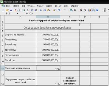
Rice. 2. Calculations of the internal investment turnover rate

1. Consider this example for all combinations of input data. To create a script, use the Tools | Scripts | Add button (Fig. 3). After clicking the OK button, it becomes possible to enter new values ​​for the cells being changed (Fig. 4).

To save the results for the first scenario, there is no need to edit the cell values ​​- just click OK (to confirm the default values ​​and exit to the Scenario Manager window).

Rice. 3. Adding a script for a combination of input data

Rice. 4. Window for changing cell values

3. To add new scenarios to the task under consideration, just click the Add button in the Scenario Manager window and repeat the above steps, changing the values ​​in the source data cells (Fig. 5).

Scenario "Turnover Rate 1" corresponds to the data (-700, 70, 90, 300; 250; 300), Scenario "Turnover Rate 2" - (-600, 50, 100, 200, 200, 300),

Scenario "Turnover Rate 3" - (-650, 90; 120; 200; 250; 250).

By clicking the Output button, you can view it on the worksheet

calculation results for the corresponding combination of initial values.

Rice. 5. Script Manager window with added scripts

4. To receive a final report on all added scenarios, click the Report button in the scenario manager window. In the script report window that appears, select the required report type and provide links to the cells in which the resulting functions are calculated. When you click OK, a report on the scenarios is displayed on the corresponding sheet of the workbook (Fig. 6).

Rice. 6. Report on scenarios for calculating the investment turnover rate

3.2. Building charts

For submission to graphically These worksheets (tables) use diagrams. The worksheet data that is used to create the charts is connected to the chart, and when it changes, the chart is updated. You can create an embedded chart, added directly to a worksheet, or run it on separate sheet diagrams in the workbook. Once created, you can customize your chart with titles and gridlines. You can use auto formats to change the chart format.

To create a chart using the Chart Wizard: the following actions:

1. Select the data you want to use in the chart.

2. Execute the Insert / Chart command or click the Chart Wizard button.

3. The Chart Wizard (step 1 of 4) dialog box appears. Select a chart type from the appropriate list, and then select a chart type. Then click on the Next> button. You have the opportunity to see a preview of the chart by left-clicking on the View result button.

Rice. 9. - Chart Wizard

4. If the range address in the Range text box of the Data Range tab is correct for the Next> button. Otherwise, select the range in the working window or enter the addresses of its cells and then click the Next> button. You can make some changes by selecting the Row tab. A new dialog box will appear.

5. In this window, you can improve the diagram using the appropriate tabs. For example, a histogram might look like this. Click the Next> button. The final Diagram Wizard window appears.

6. Specify the location of the chart.

7. Click the Finish button. The diagram appears on the worksheet.

After you insert a chart into a worksheet, you can resize it or move it to another location by first selecting it. To select a chart, place the mouse cursor on it and left-click. In this case, a thin rectangular frame will appear near the diagram with markers in the form of black squares in the corners, in the middle of each side (dimensional markers).

To resize the chart, do the following:

1. Select a chart.

2. Resize the chart by moving the size markers. To change dimensions proportionally, move the corner dimension markers; to change the width or height, move the corresponding markers in the middle of the sides.

Rice. 10. - Chart Wizard, Data Source

Figure 11. - Chart Wizard, chart parameters

spreadsheet script diagram

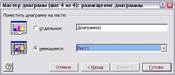
Figure 12. - Chart Wizard, chart placement

Figure 13. - Moving the diagram

IV . Workplace organization

Hardware

Computer Pentium (R) Dual - Core CPU E 5300

2.6 GHz, 0.99 GB RAM

Software

1. Operating system Microsoft Windows XP Professional

Service Pack 3

1. Microsoft Office 2013

V . Occupational safety while working with a PC

General requirements security

This instruction applies to personnel operating the equipment. computer technology And periphery equipment. The instructions contain general instructions for the safe use of electrical equipment in an institution. Requirements of this instruction are mandatory, deviations from it are not allowed. Only specially trained personnel who are at least 18 years old and fit for health reasons and qualifications to perform the specified work are allowed to operate electrical equipment independently.

Safety requirements before starting work

Before starting work, you should make sure that the electrical wiring, switches, plug sockets, with the help of which the equipment is connected to the network, the presence of grounding of the computer, its operability.

Safety requirements during operation

To reduce or prevent the influence of hazardous and harmful factors sanitary rules and regulations must be observed. Hygienic requirements for video display terminals, personal electronic computers and work organization (Approved by Resolution of the State Committee for Sanitary and Epidemiological Supervision of Russia dated July 14, 1996 N 14 SanPiN 2.2.2.542-96), and Appendix 1.2

To avoid damage to the wire insulation and the occurrence of short circuits It is not allowed to: hang anything on wires, paint or whitewash cords and wires, lay wires and cords behind gas and water pipes, behind batteries heating system, pull out plug from the outlet by the cord, force must be applied to the body of the plug.

To exclude damage electric shock It is prohibited to: frequently turn on and off the computer unnecessarily, touch the screen and the back of the computer units, work on computer equipment and peripheral equipment with wet hands, work on computer equipment and peripheral equipment that have damage to the integrity of the case, damaged wire insulation, faulty power-on indication, with signs electrical voltage on the case, place foreign objects on computer equipment and peripheral equipment.

It is prohibited to clean electrical equipment from dust and dirt while under voltage.

It is prohibited to check the functionality of electrical equipment in rooms that are not suitable for use with conductive floors, damp, and do not allow accessible metal parts to be grounded.

It is unacceptable to carry out repairs on computers and peripheral equipment while under voltage. Repair of electrical equipment is carried out only by specialist technicians in compliance with the necessary technical requirements.

To avoid electric shock, when using electrical appliances, you must not simultaneously touch any pipelines, heating radiators, or metal structures connected to the ground.

Take special care when using electricity in damp areas.

Safety requirements in emergency situations

If a malfunction is detected, immediately turn off the power to the electrical equipment and notify the administration. Continued operation is only possible after the fault has been eliminated.

If a broken wire is discovered, you must immediately inform the administration about it and take measures to prevent people from coming into contact with it. Touching the wire is life-threatening.

In all cases of electric shock to a person, call a doctor immediately. Before the doctor arrives, you need to begin providing first aid to the victim without wasting time.

It is necessary to immediately begin artificial respiration, the most effective of which is the mouth-to-mouth or mouth-to-nose method, as well as external cardiac massage.

Artificial respiration is performed for the person affected by the electric current until the doctor arrives.

It is prohibited to have flammable substances in the workplace

The following is prohibited on the premises:

a) light a fire;

b) turn on electrical equipment if the room smells of gas;

c) smoke;

d) dry something on heating devices;

d) close ventilation holes in electrical equipment

Sources of ignition are:

a) spark due to static electricity discharge

b) sparks from electrical equipment

c) sparks from impact and friction

d) open flame

If a fire hazard or fire occurs, personnel must immediately take necessary measures to eliminate it, simultaneously notify the administration about the fire.

Premises with electrical equipment must be equipped with fire extinguishers of the OU-2 or OUB-3 type.

Safety requirements after completion of work

After finishing work, it is necessary to turn off the power to all computer equipment and peripheral equipment. In case of continuous production process Only essential equipment should be left turned on.

VI. Bibliography

1. "Data Analysis in Excel" - Ginger Simon: publishing house - "Dialectics", 2004.
2. "Microsoft Office Excel for students" - L.V. Rudikov: publishing house - "BHV-Petersburg"; 2005
3. Simonovich S., Evseev G. "Excel". - "M.: INFRA M", 1998..
4. "Training. Excel 2000." - M.: Publishing house "Media", 2000.
5. "Fundamentals of Computer Science: Textbook" / A.N. Morozevich, N.N. Govyadinova and others; Ed. A.N. Morozevich. - Mn.: “New Knowledge”, 2001.
6. Langer M . "Microsoft Office Excel 2003 for Windows." - "NT Press" - 2005.
7. Verlan A.F., Apatova N.V. Informatics, -K., Kvazar-Micro, 1998..
8. The latest encyclopedia of the personal computer 2000. -2nd ed., Revised. and additional -M.: OLMA-PRESS, 2000. -p.394-430.
9. Rudenko V.D., Makarchuk A.N., Patlanzhou N.A. Practical course Informatics / ed. Maziona, -K., Phoenix, 1997.
10. Self-instruction manual for working on personal computer/ ed. Kovtanyuk Yu.S., Solovyana S.V. - K: Junior, 2001. - pp. 231-304.
11. Simonovich S.V., Evseev G.A., Alekseeva A.G. Special computer science: Tutorial. - M.: AST-PRESS: Inforkom-Press, 1999.
12. Official site Microsoft Corp. on the Internet: http://www.microsoft.com/rus

Other similar works that may interest you.vshm>
237.		Creating macros and using them in Excel	403.86 KB
	Creating macros and their use in Excel Questions covered: The concept of a macro. Purpose of the macro graphic images. Concept of a macro Before we start writing programs in VB, let's take advantage of a simple opportunity to create a macro program in VB using McroRecorder. In addition, the created macro code can serve as the basis for further development.
19515.		Practical application of motivation theory in an organization	319.27 KB
	Problems of labor motivation at Kazakh enterprises. The main thing in management is to encourage workers to develop their abilities for more intensive and productive work. To achieve this goal, the following tasks were solved in the work: Based on the goal, we can formulate the main objectives of this study: study theoretical foundations And modern trends labor motivation and its role in increasing the efficiency of the enterprise; analysis of the effectiveness of the motivation system at JSC BTA Mortgage...
20220.		Practical application of expert systems in economics	262.87 KB
	20 Practical use expert systems in economics 26 Historical aspects and evolution of expert systems 26 Expert systems economic analysis of diagnostics and forecasting of situations.33 Review of examples of expert systems in economics and computer systems. Expert systems deal with objects real world operations with which usually require significant human experience. Expert systems have one big difference: They are not intended for...
4777.		VIKNO EXCEL PROGRAMS	146.22 KB
	Operations with sheets Basic operations are associated with work sheets in the context menu that opens after right-clicking the mouse tab. You can use the following commands: Add Insert View Delete Rename Renme Move Copy Move or Copy See all sheets Select ll Sheets and so on For example, a task of the type of arkush is what is inserted: arkush Worksheet Diagram Chrt Macro MS Excel. Select the type of arch that is inserted.
4776.		TABLE LINES IN EXCEL	39.01 KB
	Table creation is one of the most powerful features of MS Excel for analyzing the data of placements in tables and lists. Creating tables manually when analyzing data for a number of reasons: Allows you to create additional tables to allow grouping of similar data, summarizing bags, and summarizing statistical characteristics of records...
3861.		PREPARING A TEST IN MS EXCEL	256.43 KB
	PREPARING A TEST IN MS EXCEL, On Sheet 1 we will type the questions and on Sheet 2 we will place the answer options, the list of answers should be vertical, the first answer empty so that after the first student’s answer the test can be returned to its original position i. Fill in the fields: Click OK and in cell D1 the following function will be inserted: The meaning of the function is as follows: If the answer in the tested cell C1 coincides with the correct one, then put 1 point in cell D1, otherwise 0 in in this case The correct answer will be has noticeably deteriorated; it has a serial number of 2 because answer No. 1 is empty. 1...
1577.		Search for lists in EXCEL	1.93 MB
	Having defined the range as a list, you can add data to the list and analyze them independently from other data within the list. For example, if you don’t have enough data in the list, you can filter the options, add a row of bags, and create a table of the results. Having defined the range as a list, you can add data to the list and analyze them independently from other data within the list.
21340.		Practical research in municipal educational institution secondary school No. 2 r. Ekaterinovka village, Ekaterinovsky district	274.54 KB
	Institute social work in the education system: theoretical aspect. Regulatory and Legal Framework Historical aspect of the organization of social work in educational institutions. Regulatory acts as the basis of social work in the education system. Essential characteristics of social work in the education system.
7166.		Purpose of spreadsheets. Introduction to MS Excel	76.37 KB
	At the bottom of the book window there are sheet shortcuts and scroll buttons, and at the top there is a title bar. In addition, the window contains sheets and scroll bars. The two middle buttons scroll one tab left or right. The listed scroll buttons and tab split marker do not activate workbook sheets.
20180.		Chart options and objects in Microsoft Office Excel	1.01 MB
	Diagrams allow you to: display data more clearly, make it easier to perceive, help with analysis and comparison, observe changes in values. And for analysis it is convenient to use diagrams with their special features. The result of the spreadsheet processor is a document in the form of a table or chart.

Microsoft Office Excel is a spreadsheet program that allows you to store, organize and analyze information. You may be under the impression that Excel is only used by a certain group of people to do certain things. complex tasks. But you are wrong! In fact, anyone can master this excellent program and use all its power to solve exclusively their everyday problems.

Excel- This universal program, which allows you to work with various formats data. In Excel you can maintain home budget, perform both simple and very complex calculations, store data, organize various diaries, draw up reports, build graphs, charts and much, much more.

Excel program is part of the Microsoft Office suite, which consists of a whole set of products that allow you to create various documents, spreadsheets, presentations and more.

In addition to Microsoft Excel, there is also whole line similar programs, which are also based on working with spreadsheets, but Excel is by far the most popular and powerful of them, and is rightfully considered the flagship of this direction. I dare say that Excel is one of the most popular programs at all.

What can I do in Excel?

Microsoft Excel has many advantages, but the most significant is, of course, its versatility. Options Excel applications are almost limitless, therefore, the more knowledge you have on this program, the larger number you can find applications for it. The following are possible areas of application for Microsoft Office Excel.

1. Working with Numeric Data. For example, drawing up a wide variety of budgets, ranging from home budgets, as the simplest, to the budget of a large organization.
2. Work with text. A diverse set of tools for working with text data makes it possible to present even the most complex text reports.
3. Creating graphs and charts. A large number of tools allows you to create a wide variety of chart options, which makes it possible to present your data in the most vivid and expressive way.
4. Creating diagrams and drawings. In addition to graphs and charts, Excel allows you to insert many different shapes and SmartArt graphics into your worksheet. These tools significantly increase the data visualization capabilities of the program.
5. Organizing Lists and Databases. Microsoft Office Excel was originally designed with a structure of rows and columns, so organizing work with lists or creating a database is an elementary task for Excel.
6. Data import and export.Excel allows you to exchange data with the most various sources, which makes working with the program even more universal.
7. Automation of similar tasks. Using macros in Excel allows you to automate the execution of the same type of time-consuming tasks and reduce human participation to a single mouse click to run the macro.
8. Creating Control Panels. In Excel, you can place controls directly on the worksheet, which allows you to create visual, interactive documents.
9. Built-in programming language. Built into a Microsoft app Excel language Visual programming Basic for Applications (VBA) allows you to expand the program's capabilities at least several times. Knowledge of a language opens up completely new horizons for you, for example, creating your own custom functions or entire add-ons.

Possibilities Excel applications The list could go on for a very long time; above I presented only the most basic of them. But it is already clear to see how useful knowledge of this program will be for you.

Who is Excel made for?

Initially Excel program was created exclusively for office work, since only an organization could afford such a luxury as a computer. Over time, computers began to appear more and more in homes ordinary people, and the number of users gradually grow. On this moment Almost every family has a computer and most of them have it installed Microsoft package Office.

There are hundreds of companies in Russia offering Microsoft Office courses. Excel is taught in educational institutions, hundreds of books and training courses have been published on Excel. Knowledge of Office is required when applying for a job or this knowledge is counted as additional benefit. All this suggests that knowledge office programs, in particular Excel, will be useful to everyone without exception.

Microsoft Excel- This component Microsoft Office. Excel was introduced in 1987. The spreadsheet is one of the most convenient applications to process data and present it in tabular form. Programs that process spreadsheets are called table processors. Excel allows you to analyze data using charts, create document forms, and make calculations using formulas. For people, professional activity which is associated with numbers, drawing up reports and forms, and analyzing these results, the program is an indispensable assistant. With its help, they can keep a log of business transactions, issue an invoice, payroll, staffing table or invoice, and perform any other tasks related to systematization and organization of information. The name of the program is short for the English word Excellent - which means “excellent”.

The Excel menu consists of:

2. Editing - can be used when editing a document. It contains the commands Undo, Cut, Copy, Paste, Find, Fill, Go. Selecting the Undo command allows you to discard the formatting, copying or deleting that was just performed, i.e. any action the result of which you are not happy with. The Cut, Copy and Paste commands can be used to fill cells with data, and the Go To command is used to move to a cell with a specific address.

3. The Insert menu item contains the commands Rows, Sheet, Chart, Functions, Note. As the name suggests, you can use the commands on this menu to add rows, sheets, and charts, as well as to insert functions into your document when creating formulas and notes.

4. The Format menu item contains commands that can be used when formatting cells.

5. The Data menu item is used when working with databases. Commands Sort, Filter, Pivot table allows you to sort database tables, select data from them according to certain criteria, and create pivot tables.

6. The Service menu item is used to configure the program.

In Excel, row and column numbers are called headings, and cell numbers are called cell names. The cell in which the user is working is called active and is highlighted with a bold frame. The name of the active cell is displayed in the upper left side Excel windows, this field is called the name field. If we want to get a product in any cell (for example, calculating the cost of some parts quantity * price) - we do it as follows: activate this cell (where the result will be) → Standard toolbar → Insert functions → Function Wizard dialog box in on the left side of the window, in the category section, select Mathematical functions and looking for a WORK. After selection required function and clicking OK, a second window of the Function Wizard opens - in which you need to specify the product of which two (or more) cells we need. Cells are listed using: (colon). Next, the formula needs to be set for the entire column, for this we use Autofill. The active cell is marked with a bold rectangle, and in the lower right corner there is bold point. This point is called autocomplete marker. If you place the mouse pointer on this marker, it will turn into a black cross. We make active a cell in which there is already a formula, move the pointer to the autofill marker, click the left button and, without releasing it, “stretch” the frame of the active cell down to the last line we filled in. We release the mouse button and see that the column is filled with data. Now let's make cell G 19 active, click on the button Σ Autosum, which is located on Standard panel tools to the left of the Insert Functions button. To select cells, click the left button and, without releasing, “stretch” the cell to the last row we need. In the formula bar and in cell G 19 itself you can see the formula (SUM(G 7:G 17)), press Enter and the result is obtained in the cell. Excel allows you to specify what kind of data is stored in cells, this is called number formats. The set of all cell settings is called cell format.

Menu Format, select the item Cells, in the dialog box on the first tab Number In the Number formats field, select Currency, you can specify how many decimal places we want to see. After selecting the format OK. After this, the PRICE and AMOUNT numbers will be displayed in monetary terms. The table is ready, but when printed, the cell borders will not be displayed. If we want to show these borders, we need to use framing tools. To do this, use the button Borders. After framing and filling, the table will look like this: printed form just like on the monitor screen.

Selecting a column/row. To select a column or row, just click on the heading of the desired column or row. If you need to select several consecutive columns or rows, then you need to click on the heading of the first desired column/row and, without releasing the button, drag the pointer over the headings that we need. If some of the selected rows or columns did not need to be selected, you can selectively deselect (or select) using the Ctrl key.

Changing column/row width/height. The change is made by the pointer when it accepts a double-headed arrow.

Inserting rows/columns/cells. If during work there is a need to insert rows or columns into the table, we will do it as follows:

¯ select the row above which you want to add a new one in the table

¯ right-click on the selection and in the context menu that opens, select Add Cells.

Delete rows/columns/cells. To delete rows or columns, you must first select them. You can delete either a single row or a group of rows or columns. Select by clicking the left mouse button, “stretch” until we mark everything that needs to be deleted, press the right mouse button and select the item in the context menu Delete. Select the deletion method in the window (shift left or up).

Excel sheets. Excel Documents- this is not a single table, which we have been working with so far, but a workbook, which by default contains three such tables. These tables are called sheets. It's easy to move from sheet to sheet; there are sheet shortcuts in the lower left corner. When working with complex documents, sheets are very convenient to use, since from any sheet you can make links to cells of other sheets and use data from several sheets when creating formulas.

Sheet formatting. You can change the appearance of the data you enter. Change appearance document is called formatting the sheet or cells. For formatting, use the panel located under the title of the program window, or the Format→Cells command from the menu bar. Cells must first be selected. You can also use the Format Cells context menu command to open the Format Cells dialog box.

Sample format. To copy the cell format from one sheet to another, use the button Sample format. The point of copying a format is to transfer only the format of the selected cell to another cell, leaving its contents the same. The same is true for a group of cells.

1. Select a fragment formatted appropriately and click the Format As Sample button. A brush icon will appear next to the mouse pointer.

2. Select the cell or range to which you want to apply the selected format.

3. Release the mouse button. The selected cells will be formatted as expected.

Exercise 1.

In cells A1-A3, enter the number 20 and assign the cells the formats General, Cash, Interest

2000%, center the numbers

Exercise 2.

Open Sheet 2, in cell with address A4 enter the value Departure, in cell A5 the value Arrival. To make the data in cells look beautiful, you can use the Format→Column→Auto-Fit Width command. In cells B4 and B5, indicate the dates of departure and return from the business trip. Let it be 01/10/2004 and 01/16/2004. In the cell with the address B6, enter the formula for calculating the days of stay on a business trip: = B5 - B4.

Building charts. A diagram is one way of presenting data. The point of diagrams is to more clearly present the information contained in the table. Information presented in graphical form is much easier to perceive in pictures than in text or tabular form. How to create a chart in Excel - you need to select the data for the chart and launch the Chart Wizard. KK and all others Microsoft Wizards Office this wizard will ask you a series of questions to determine your settings created object, and then creates it according to the instructions received. Chart Wizard on the toolbar, or the menu command Insert→Diagram. In Excel you can create 3D and 2D charts. By default, the diagram is built over the entire selected area. If in top line and there is text in the left column, the program automatically generates a legend based on them. Legend is a description symbols adopted in this diagram. After creation, the diagram can be edited: change the colors of the lines and columns, and the font of the inscriptions on the diagram. To do this, you need to switch to the diagram editing mode by double-clicking on one of the diagram elements.

Exercise 3.

Sale of goods.

A1 - title of the diagram - by warehouse

A3 - wholesale warehouse

A4 - general warehouse

Q2 - 2 - Quarter 1 - Quarter 3. - use the auto-fill option.

Fill the table with data, select cells and launch the Chart Wizard. To analyze quarterly sales, it is convenient to use a pie chart.

To analyze sales for a wholesale warehouse, mark cells A2:E2

For general warehouse A3:E3

Examples of using Excel

Registration of the transaction log

Filling out A1 - transaction log

B2 - Business transaction

C2 - Debit

D2 - Credit

E2 - Amount

Resize cell B2 so that the text is fully visible. Select cells A2-E2 and format them using bold style, font size 14. Align the cells to the center, highlight them with color (use the formatting toolbar buttons). Select cells A1-E1 and click on the button Combine and place in the center on the formatting toolbar. The title should be in the center of the magazine. Fill the log with data. If a business transaction spans several lines, select Format→Cells→Alignment tab and check the Wrap by words box (there are three boxes, check the box you want). The numbers can be aligned to the center of the cell; to do this, click on the Center button, having first selected the cells, starting with E3. Format these cells by selecting the Currency format. To do this, Format→Cells→Number, set the format to Currency in the Number Formats field and enter the value 2 in the Number of Decimal Places field. Similarly, the Excel program can be used to prepare payroll statements, invoices, and balance sheets. Certainly, we're talking about o use Excel for these forms if the enterprise is small and reporting on it is not too cumbersome.

Introduction

1: Microsoft Excel

2: Data analysis. Using Scripts

2.1 Data analysis in MS Excel

2.2 Scenarios

Conclusion

Bibliography

Introduction

Microsoft Office, the most popular office family software products, includes new versions of familiar applications that support Internet technologies, and allow you to create flexible Internet solutions

Microsoft Office is a family of software Microsoft products, which brings together the world's most popular apps into unified environment, ideal for working with information. Microsoft Office includes a word processor Microsoft Word, Microsoft Excel spreadsheets , Microsoft Power Point presentation tool and the new Microsoft Outlook application . All of these applications make up the Standard Edition of Microsoft Office. IN Professional editorial staff Microsoft Access DBMS is also included.

Microsoft Excel– a program designed to organize data in a table for documenting and graphically presenting information.

Program MS Excel is used when creating complex documents in which it is necessary:

use the same data in different worksheets;

change and restore connections.

The advantage of MS Excel is that the program helps to operate with large volumes of information. MS Excel workbooks provide the ability to store and organize data, and calculate the sum of values ​​in cells. Ms Excel provides a wide range of methods to make information easy to understand.

Workbookis a setworksheets, each of which has a table structure. The document window displays only the current (active) worksheet with which you are working. Each worksheet has a title, which appears on the worksheet tab at the bottom of the window. Using shortcuts, you can switch to other worksheets included in the same workbook. To rename a worksheet, you need to double-click on its tab and replace the old name with a new one or by executing the following commands: menuFormat, line Sheet in the menu list, Rename. Or you can place the mouse pointer on the active worksheet shortcut, right-click, and then click on the line in the context menu that appearsRenameand perform a rename. You can add (insert) new sheets to the workbook or delete unnecessary ones. Inserting a sheet can be done by executing the menu commandInsert, line Sheetin the list of menu items. The sheet will be inserted before the active sheet. The above actions can also be performed using the context menu, which is activated by clicking the right mouse button, the pointer of which should be placed on the tab of the corresponding sheet. To swap worksheets, you need to place the mouse pointer on the tab of the sheet being moved, press the left mouse button and drag the tab to the desired location.

Worksheet(table) consists of rows and columns. The columns are headed with capital Latin letters and, further, with two-letter combinations. The worksheet contains a total of 256 columns, named A through IV. The lines are numbered sequentially from 1 to 65536.

At the intersection of columns and rows,cellstables. They are the minimum elements designed to store data. Each cell has its own address.Addresscell consists of the column name and row number at the intersection of which the cell is located, for example, A1, B5, DE324. Cell addresses are used when writing formulas that define the relationship between values ​​located in different cells. At the current time, only one cell can be active, which is activated by clicking on it and highlighted with a frame. This frame acts as a cursor in Excel. Data entry and editing operations are always performed only in the active cell.

Data located in adjacent cells that form a rectangular area can be referenced as a single unit in formulas. A group of cells bounded by a rectangular area is calledrange. The most commonly used rectangular ranges are formed at the intersection of a group of sequential rows and a group of sequential columns. A range of cells is indicated by specifying the address of the first cell and the address of the last cell in the range, separated by a colon, for example, B5:F15. Selecting a range of cells can be done by dragging the mouse pointer from one corner cell to the opposite cell diagonally. The frame of the current (active) cell expands, covering the entire selected range.

To speed up and simplify computational work, Excel puts at the user's disposal a powerful apparatus of worksheet functions that allow almost all possible calculations to be carried out.

In total, MS Excel contains more than 400 worksheet functions (built-in functions). All of them, according to their purpose, are divided into 11 groups (categories):

financial functions;

date and time functions;

arithmetic and trigonometric (mathematical) functions;

statistical functions;

functions of links and substitutions;

database functions (list analysis);

text functions;

logical functions;

information functions (checking properties and values);

engineering functions;

external functions.

Writing any function into a worksheet cell must begin with the equals symbol (=). If a function is used as part of any other complex function or in a formula (megaformula), then the equal symbol (=) is written before this function (formula). Any function is accessed by specifying its name followed by an argument (parameter) or a list of parameters in parentheses. The presence of parentheses is mandatory; they serve as a sign that the name used is the name of a function. List parameters (function arguments) are separated by semicolons (;). Their number should not exceed 30, and the length of a formula containing as many calls to functions as desired should not exceed 1024 characters. When writing (entering) a formula, it is recommended to type all names in lowercase letters, then correctly entered names will be displayed in capital letters.

1.4 Possible errors when using functions in formulas

When working with spreadsheets, it is important not only to know how to use them, but also to avoid making common mistakes.

Research has shown that more than half of the people who frequently use Microsoft Excel in their work keep a regular calculator on their desktop! The reason turned out to be simple: in order to perform the operation of summing two or more cells to obtain an intermediate result (and, as practice shows, most people have to perform such an operation quite often), it is necessary to perform two extra steps. Find the place in the current table where the total amount will be located and activate the summation operation by pressing the S (sum) button. And only after this you can select those cells whose values ​​are supposed to be summed.

In an Excel cell, you may see ####### (hash marks) instead of the expected calculated value. This is just a sign that the cell width is not sufficient to display the resulting number.

Excel displays the following values, called error constants, in cells that contain formulas when errors occur in the calculations of those formulas:

2. Data analysis. Using Scripts

2.1 Data analysis

Data- information:

Obtained by measurement, observation, logical or arithmetic operations;

Presented in a form suitable for permanent storage, transmission and (automated) processing.

IN Excel data type– type, value stored in the cell.

When data is entered into a worksheet, Excel automatically analyzes it to determine the data type. The default data type assigned to a cell determines the data analysis that can be applied to that cell.

For example, most data analysis tools use numerical values. If you try to enter a text value, the program will respond with an error message.

Data types:

Text

Numerical

Number

Numeric characters

Fractions

date and time

Time

Formulas

Data analysis - a field of computer science that deals with the construction and research of the most general mathematical methods and computational algorithms for extracting knowledge from experimental (in a broad sense) data.

Data analysis – comparison of various information.

Working with a table is not limited to simply entering data into it. It is difficult to imagine an area where analysis of this data would not be required.

Data tables are part of a block of tasks that are sometimes called what-if analysis tools. A data table is a range of cells that shows how changing certain values ​​in formulas affects the results of those formulas. Sheets provide a way to quickly calculate multiple versions in a single operation, and a way to view and compare the results of all the different versions on a single worksheet.

Ms Excel provides ample opportunities for analyzing the data in the list. Analysis tools include:

2.2 Scenarios

One of the main benefits of data analytics is predicting future events based on today's information.

Scripts are part of a task block, sometimes called tools.what-if analysis (What-if analysis. The process of changing cell values ​​and analyzing the effect of those changes on the result of a formula calculation on a worksheet, such as changing the interest rate used in a depreciation table to determine payment amounts.).

Scenario is a set of values ​​that are stored in the Microsoft Office Excel application and can be automatically inserted into the worksheet. Scenarios can be used to predict the results of worksheet calculation models. It is possible to create and save different groups of values ​​in a worksheet, and then switch to any of these new scenarios to view different results. Or you can create multiple input data sets (changeable cells) for any number of variables and give each set a name. Based on the name of the selected data set, MS Excel will generate the analysis results on the worksheet. In addition, the scenario manager allows you to create a final report on scenarios, which displays the results of substitution of various combinations of input parameters.

As you develop the scenario, the data on the sheet will change. For this reason, before you start working with the script, you will have to create a script that saves the original data, or create a copy of the Excel sheet.

All scripts are created in the dialog box Adding a script. First, you need to specify the cells to display the predicted changes. Cell references are separated from each other by a colon or semicolon. Then in the dialog box Scenario cell meaning each cell is assigned a new value. These values ​​are used when the corresponding script is executed. After entering the values, a script is generated. When you select another scenario, the values ​​in the cells change as specified in the scenario.

To protect the script, checkboxes are used that are placed at the bottom of the dialog box Adding a script. Checkbox Deny changes does not allow users to change the script. If the checkbox is activated Hide, then users will not be able to open the sheet and see the script. These options only apply when sheet protection is set.

If you need to compare several scenarios at the same time, you can create Final report, by clicking the button in the dialog box Report.

In many economic problems, the calculation result depends on several parameters that can be controlled.

The script manager is opened with the command Service/Scripts(Fig. 1). In the scenario manager window, using the appropriate buttons, you can add a new scenario, change, delete or display an existing one, as well as combine several different scenarios and get a final report on existing scenarios.

2.3 Example of calculating the internal investment turnover rate

Initial data: Project costs amount to 700 million rubles. Expected income over the next five years will be: 70, 90, 300, 250, 300 million rubles. Also consider the following options (project costs are presented with a minus sign):

600; 50;100; 200; 200; 300;

650; 90;120;200;250; 250;

500, 100,100, 200, 250, 250.

Figure 1. Scenario Manager window

Solution:

To calculate the internal rate of investment turnover (internal rate of return), the function is usedVSD (in earlier versions - inhale):

VSD - Returns the internal rate of return for a series of cash flows, represented by their numerical values. These cash flows do not have to be equal in size, as in the case of an annuity. However, they must take place at regular intervals, such as monthly or annually.

Internal rate of return is the interest rate accepted for an investment consisting of payments (negative values) and income (positive values) that are made in successive periods of equal duration.

VSD ( Values ; Assumptions )

Assumption is a value that is assumed to be close to the VSD result.

In our case, the function to solve the problem uses only

argumentValues , one of which is necessarily negative (project costs). If the internal investment turnover rate is greater than the market rate of return, then the project is considered economically feasible. Otherwise, the project must be rejected.

The solution is shown in Fig. 2. Formulas for calculation:

in cell B14:

VSD(B5:B10)

in cell C14:

IF(B14>B12);"The project is economically feasible";

"The project must be rejected")

Figure 2. Calculation of the internal investment turnover rate

2. Consider this example for all combinations of input data. To create a script you should use the commandService | Scenarios | buttonAdd (Fig. 3). After pressing the buttonOK it becomes possible to enter new values ​​for the cells being changed (Fig. 4).

To save the results of the first scenario, there is no need to edit cell values ​​- just click the buttonOK ( to confirm the default values ​​and exit to the windowScript Manager.

Fig 3. Adding a script for a combination of source data

Fig 4. Window for changing cell values.

3. To add new scenarios to the task under consideration, just click the buttonAdd in the window Script Manager and repeat the above steps, changing the values ​​in the source data cells (Fig. 5).

Scenario " Turnover speed 1 " corresponds to the data (-700; 70; 90; 300; 250; 300), Scenario "Turnover speed 2 » - (-600; 50; 100; 200; 200; 300),

Scenario " Turnover speed 3 » - (-650; 90; 120; 200; 250; 250).

Pressing the button Withdraw, can be viewed on the worksheet

calculation results for the corresponding combination of initial values.

Fig 5. Script Manager window with added scripts

4. To receive a final report for all added scenarios, click the buttonReport in the Script Manager window. In the scenario report window that appears, select the required report type and provide links to the cells in which the resulting functions are calculated. When you press the buttonOK A report on the scenarios is displayed on the corresponding sheet of the workbook (Fig. 6).

Figure 6. Report on scenarios for calculating the investment turnover rate

Conclusion

Characteristic feature modernity is rapid scientific and technological progress, which requires managers and businessmen to significantly increase responsibility for qualitydecision making. This is the main reason that necessitates scientific decision-making.

Using this product you can analyze large amounts of data. In Excel, you can use more than 400 mathematical, statistical, financial and other specialized functions, link various tables to each other, choose arbitrary data presentation formats, and create hierarchical structures.

MS Excel, being a leader in the market for spreadsheet processing programs, determines development trends in this area. Up until version 4.0, Excel was the de facto standard in terms of functionality and usability. Now there are much newer versions on the market that contain many improvements and pleasant surprises.

Bibliography

Official website of Microsoft Corp. on the Internet: http://www.microsoft.com/rus

"Data analysis inExcel" - Ginger Simon: publishing house - “Dialectics”, 2004.

« MicrosoftOfficeExcelfor the student" - L.V. Rudikova: publishing house - “BHV-Petersburg”; 2005

Simonovich S., Evseev G. “Excel”. – “M.: INFRA-M”, 1998.

"Education. Excel 2000". – M.: Publishing house “Media”, 2000.

“Fundamentals of Computer Science: Textbook. Benefit" / A.N. Morozevich, N.N. Govyadinova and others; Ed. A.N. Morozevich. – Mn.: “New Knowledge”, 2001.

Langer M . "Microsoft Office Excel 2003 For Windows". – “ NT Press " – 2005.

Program description

Microsoft Excel is widely used computer program, with the help of which calculations are made, tables and diagrams are compiled, simple and complex functions are calculated.

This program is included in the Microsoft Office package, and therefore is installed on almost all computers. The ability to create tables, charts and reports, creating the most complex calculations makes this program popular among accountants and economists. However, the program is different clear interface and ease of use.

At its core, Microsoft Excel is big table, intended for entering data into it. The program's functions allow you to carry out almost any manipulation with numbers. The spreadsheet is the main tool that is used for processing and analysis digital information using computer technology.

At the same time, in addition to numerical and financial operations, Microsoft Excel can be used in the process of data analysis, opening up wide opportunities for users for convenient automation and data processing.

The peculiarity of the program is that it allows complex calculations. That is, during the calculation process, you can simultaneously operate with data that is located in different zones spreadsheet and at the same time connected by a certain dependence. Such calculations are carried out thanks to the ability to enter various formulas into table cells. After the calculation is completed, the result will be displayed in the cell with the formula. The available range of formulas includes different functions– from addition and subtraction to calculations related to finance or statistics.

An important feature of using a spreadsheet is that results are automatically recalculated if cell values ​​change. Excel can be used when performing financial calculations, accounting and monitoring the personnel of a particular organization, and in constructing and updating charts that are based on entered numbers.

The file with which it is supposed Excel work, is called a book. It includes several worksheets that can contain a variety of data, ranging from tables and texts to diagrams and pictures. Microsoft Excel is designed to support and use XML formats, and can also open formats such as CSV, DBF, SYLK, DIF.