Creating a Spreadsheet in Excel

Program Microsoft Excel designed for working with data tables, mainly numeric. When creating a table, you enter, edit, and format text and numeric data, as well as formulas. The presence of automation tools facilitates these operations. The created table can be printed.

Spreadsheet Basics
An Excel document is called a workbook. A workbook is a collection of worksheets, each of which has a tabular structure and can contain one or more tables. In the document window in Excel, only the current worksheet is displayed, with which you are working (Fig. 12.2). Each worksheet has a title that is displayed on. sheet tab displayed at the bottom of the sheet. Using shortcuts, you can switch to other worksheets included in the same workbook. To rename a worksheet, double-click on its tab.
The worksheet consists of rows and columns. Columns are headed in capitals with Latin letters and, further, two-letter combinations. In total, the worksheet can contain up to 256 columns, numbered A through IV. Lines are numbered sequentially, from 1 to 65,536 (the maximum allowed line number).
Cells and their addressing. Table cells are formed at the intersection of columns and rows. They are the minimum elements for storing data. The designation of an individual cell combines the column and row numbers (in that order) at the intersection of which it is located, for example: A1 or DE234. The cell designation (its number) serves as its address. Cell addresses are used when writing formulas that define the relationship between values located in different cells.
One of the cells is always active and is highlighted by the active cell frame. This frame plays the role of a cursor in Excel. Input and editing operations are always performed in the active cell. You can move the frame of the active cell using the cursor keys or the mouse pointer.

Rice. 12.2. Worksheet spreadsheet Excel

Range of cells. Data located in adjacent cells can be referenced in formulas as a single unit. This group of cells is called a range. The most commonly used are rectangular ranges, formed at the intersection of a group of sequential rows and a group of sequential columns. The range of cells is indicated by indicating through a colon the numbers of cells located in opposite corners of the rectangle, for example: A1; C15.
If you want to select a rectangular range of cells, you can do this by dragging the pointer from one corner cell to the opposite one diagonally. The frame of the current cell expands to cover the entire selected range. To select an entire column or row, click on the column (row) header. By dragging the pointer over the headings, you can select multiple consecutive columns or rows.
Entering, editing and formatting data
A single cell can contain data belonging to one of three types; text, number or formula - and also remain empty. Excel when saving workbook writes to the file only the rectangular area of worksheets adjacent to the left top corner(cell A1) and containing all filled cells.
The type of data placed in the cell is determined automatically as you enter it. If this data can be interpreted as a number, Excel program does so. Otherwise, the data is treated as text. Entering a formula always begins with the “=” symbol (equal sign).
Entering text and numbers. Data is entered directly into the current cell or into the formula bar located at the top of the program window directly below the toolbars (see Fig. 12.2). The input location is marked with a text cursor. If you start typing by pressing the alphanumeric keys, the data in the current cell is replaced with the text you type. If you click on the formula bar or double-click on the current cell, the old contents of the cell are not deleted and you can edit it. In any case, the entered data is displayed both in the cell and in the formula bar.
To complete the entry and save the entered data, use the Enter button in the formula bar or the ENTER key. To cancel changes made and restore the cell's previous value, use the Cancel button in the formula bar or the ESC key. The easiest way to clear the current cell or selected range is to use the DELETE key.
Formatting cell contents. By default, text data is aligned to the left edge of the cell, and numbers are aligned to the right. To change the display format of the data in the current cell or selected range, use the Format > Cells command. The tabs of this dialog box allow you to select the format for recording data (the number of decimal places, indicating the monetary unit, how the date is written, etc.), set the direction of the text and the method of its alignment, define the font and style of characters, control the display and appearance of frames, and set the background color.

Spreadsheet calculations
Formulas. Calculations in Excel tables are carried out using formulas. A formula can contain numeric constants, cell references, and Excel functions, connected by symbols of mathematical operations. Parentheses allow you to change standard order performing actions. If a cell contains a formula, the worksheet displays the current result of that formula. If you make a cell current, the formula itself is displayed in the formula bar.
The rule for using formulas in Excel is that if the value of a cell actually depends on other cells in the table, you should always use a formula, even if the operation can easily be done in your head. This ensures that subsequent editing of the table will not violate its integrity and the correctness of the calculations performed in it.
Cell references. The formula can contain links, that is, addresses of cells whose contents are used in calculations. This means that the result of the formula depends on the number in another cell. The cell containing the formula is therefore a dependent cell. The value displayed in a formula cell is recalculated when the value of the referenced cell changes.
You can set a cell reference different ways. First, the cell address can be entered manually. Another way is to click on the desired cell or select the range whose address you want to enter. The cell or range is highlighted with a dotted frame.
All dialog boxes Excel programs that require you to specify cell numbers or ranges contain buttons attached to the corresponding fields. When you click on this button, the dialog box is minimized possible size, which makes it easier to select the desired cell (range) by clicking or dragging (Fig. 12.3).

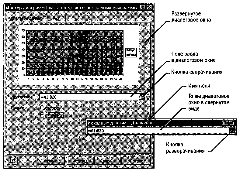
Rice. Dialog box expanded and collapsed

To edit a formula, double-click on the corresponding cell. In this case, the cells (ranges) on which the value of the formula depends are highlighted on the worksheet with colored frames, and the links themselves are displayed in the cell and in the formula bar in the same color. This makes it easier to edit and check the correctness of formulas.
Absolute and relative links. By default, cell references in formulas are treated as relative. This means that when you copy a formula, the addresses in the references automatically change according to the relative location of the original cell and the copy being created.
For example, let's say cell B2 contains a link to cell A3. In relative view, we can say that the reference points to a cell that is one column to the left and one row below the given one. If the formula is copied to another cell, then this relative reference indication will remain. For example, when you copy a formula into cell EA27, the link will continue to point to the cell to the left and below, in in this case per cell DZ28.
With absolute addressing, the reference addresses do not change when copied, so the referenced cell is treated as a non-tabular cell. To change the addressing method when editing a formula, select the cell reference and press F4. Cell number elements that use absolute addressing are preceded by a $ character. For example, when you press the F4 key successively, the cell number A1 will be written as A1, $A$ 1, A$ 1 and $A1. In the last two cases, one of the components of the cell number is treated as absolute, and the other as relative.

Copying cell contents
Copying and moving cells in Excel can be done using the drag-and-drop method or via the clipboard. When working with a small number of cells, it is convenient to use the first method; when working with large ranges, it is convenient to use the second.
Drag and drop method. To use drag-and-drop to copy or move the current cell (selected range) along with its contents, move the mouse pointer over the frame of the current cell (it will appear as an arrow). Now the cell can be dragged anywhere on the worksheet (the insertion point is marked with a tooltip).
To select the method of performing this operation, as well as for more reliable control over it, it is recommended to use special drag and drop using right button mice. In this case, when you release the mouse button, special menu, where you can select the specific operation to perform.
Using the clipboard. Transferring information via the clipboard is included in the program Excel specific features related to the complexity of control over this operation. First, you need to select the range to be copied (cut) and give the command to place it on the clipboard: Edit > Copy or Edit > Cut. Pasting data into a worksheet is only possible immediately after it is placed on the clipboard. Attempting to perform any other operation will cancel the copy or move process that was in progress. However, there is no data loss because the cut data is removed from its original location only when the insertion occurs.
The insertion location is determined by selecting a cell that corresponds to the upper left corner of the range placed on the clipboard, or by selecting a range that is exactly the same size as the one being copied (moved). Pasting is done using the Edit > Paste command. You can use the Edit > command to control how you paste. Special insert. In this case, the rules for inserting data from the clipboard are set in the dialog box that opens.

Automation of input
Since tables often contain repeated or similar data, Excel contains input automation tools. Features include AutoComplete, Number AutoFill, and Formula AutoFill.
Auto-completion. To automate text data entry, the autocompletion method is used. It is used when entering cells in one column of a worksheet. text strings, among which there are repeating ones. As you enter text data into the next cell, Excel checks that the entered characters match the strings in the column above. If a clear match is found, the entered text is automatically completed. Pressing the ENTER key confirms the autocomplete operation, otherwise you can continue entering without paying attention to the proposed option.
You can interrupt AutoComplete by leaving an empty cell in a column. Conversely, to use AutoComplete, the filled cells must be in a row, with no gaps between them.
Autofill with numbers. When working with numbers, the autocomplete method is used. In the lower right corner of the current cell frame there is a black square - a fill marker. When you hover over it, the mouse pointer (it usually looks like a thick white cross) takes the form of a thin black cross. Dragging a fill handle is considered an operation to "multiply" the contents of a cell either horizontally or vertically.
If a cell contains a number (including a date, a monetary amount), then dragging the marker copies the cells or fills them with an arithmetic progression. To select the autofill method, you must perform a special drag and drop using the right mouse button.
For example, let cell A1 contain the number 1. Hover your mouse over the fill handle, right-click, and drag the fill handle so that the frame covers cells A1, B1, and C1, and release the mouse button. If you now select the Copy cells item in the menu that opens, all cells will contain the number 1. If you select the Fill item, then the cells will contain the numbers 1, 2 and 3.
To accurately formulate the conditions for filling cells, you should give the command Edit > Fill > Progression. In the Progression dialog box that opens, select the progression type, step size, and limit value. After clicking the OK button, Excel automatically fills the cells in accordance with the specified rules.
Autofill formulas. This operation is performed in the same way as autofilling numbers. Its peculiarity is the need to copy references to other cells. During autocomplete, the nature of the links in the formula is taken into account: relative links change in accordance with the relative location of the copy and the original, absolute links remain unchanged.
For example, assume that the values in the third column of the worksheet (column C) are calculated as the sum of the values in the corresponding cells of columns A and B. Enter the formula =A1 +B1 in cell C1. Now let's copy this formula using the autofill method into all cells of the third column of the table. Relative addressing allows the formula to be correct for all cells in a given column.
Table 12.1 shows the rules for updating links when autocomplete along a row or along a column.
Table 12.1.
Rules for updating links during autocomplete

Link in source cell	Link in next cell
	When filling to the right	When filling down
A1 (relative)	B1	A2
$A1 (absolute by column)	$A1	$A2
A$1 (absolute by line)	$1	A$1
$A$1 (absolute)	$A$1	$A$1

Using Standard Features
Standard functions are used in Excel only in formulas. Calling a function consists of specifying the name of the function in the formula, followed by a list of parameters in parentheses. Individual parameters are separated in the list by semicolons. The parameter can be a number, a cell address, or an arbitrary expression, which can also be calculated using functions.
Formula palette. If you start entering a formula by clicking on the Change formula button in the formula bar, a formula palette appears under the formula bar, which has the properties of a dialog box (Fig. 12.4). It contains the value that will be obtained if you immediately finish entering the formula. A drop-down list of functions now appears on the left side of the formula bar, where the current cell number used to be located. It contains the ten most recently used functions, as well as More Functions.
Using the Function Wizard. Selecting Other Functions launches the Function Wizard to make selection easier. desired function. In the Category list, select the category to which the function belongs (if it is difficult to determine the category, use the Full alphabetical list item), and in the Function list, select a specific function of this category. After clicking the OK button, the function name is entered in the formula bar along with parentheses limiting the list of parameters. The text cursor is positioned between these brackets.

Rice. 12.4. Formula Bar and Formula Palette

Entering function parameters. As you enter function parameters, the formula palette changes appearance. It displays fields for entering parameters. If the parameter name is in bold, the parameter is required and the corresponding field must be filled in. Parameters whose names are given normal font, can be omitted. At the bottom of the palette is given short description functions, as well as the purpose of the parameter being changed.
Parameters can be entered directly into the formula bar or into fields in the formula palette, or, if they are links, selected on the worksheet. If a parameter is specified, the Formula palette shows its value, and for omitted parameters, the default values. Here you can also see the value of the function calculated by given values parameters (see Fig. 12.4).
The rules for calculating formulas containing functions do not differ from the rules for calculating more simple formulas. Cell references used as function parameters can also be relative or absolute, which is taken into account when copying formulas using the AutoComplete method.

Printing Excel Documents
The screen view of a spreadsheet in Excel is significantly different from what it would look like if the data were printed out. This is due to the fact that a single worksheet has to be divided into fragments, the size of which is determined by the format of the printed sheet. In addition, the design elements of the program's working window: row and column numbers, conventional cell boundaries - are usually not displayed when printing.
Preview. Before printing a worksheet, you must switch to preview(Preview button on standard panel instruments). The preview mode (Fig. 12.5) does not allow editing the document, but allows you to see it on the screen exactly as it will be printed. In addition, Preview mode allows you to change the printed page properties and print settings.

Rice. 12.5. Preview your document before printing

Preview mode is controlled using the buttons located along the top edge of the window. The Page button opens the Page Setup dialog box, which is used to set page parameters: sheet orientation, page scale (changing the scale allows you to control the number of printed pages required for the document), document margin sizes. Here you can set the top and footers for the page. The Sheet tab enables or disables printing of the grid, row and column numbers, and selects the pagination sequence for a worksheet that is larger than the printed page in both length and width.
You can also change the size of page margins, as well as the width of cells when printing, directly in preview mode, using the Margins button. When you click this button, markers appear on the page to indicate page margins and cell boundaries. You can change the position of these borders by dragging.
There are three ways to exit Preview mode, depending on what you plan to do next. Clicking the Close button allows you to return to editing the document. Clicking the Page Layout button returns you to document editing, but in page layout mode. In this mode, the document is displayed in such a way as to most conveniently show not the contents of the table cells, but the print area and the borders of the document pages. Switch between markup mode and normal mode can also be done through the View menu (commands View > Normal and View > Page Layout). The third way is to start printing the document.
Print the document. Clicking the Print button opens the Print dialog box, which is used to print the document (you can also open it without previewing it using the File > Print command). This window contains standard means controls used to print documents in any application.
Selecting the print area. The print area is the part of the worksheet that should be printed. By default, the print area coincides with the filled part of the worksheet and is a rectangle adjacent to the upper left corner of the worksheet and covers all filled cells. If some of the data should not be printed on paper, the print area can be set manually. To do this, select the cells that should be included in the print area and give the command File > Print Area > Set. If only one cell is current, the program assumes that the printable area is simply not selected and displays a warning message.
If the print area is specified, the program displays it in preview mode and prints only that area. The boundaries of the printable area are highlighted on the worksheet with a large dotted line (solid line in markup mode). To change the print area, you can set new area or use the File > Print Area > Remove command to return to the default settings.
The boundaries of individual printed pages are displayed on the worksheet as small dotted lines. In some cases it is required that specific cells were placed together on the same printed page or, conversely, the separation of printed pages occurred at a certain place on the worksheet. This feature is achieved by manually setting the boundaries of printed pages. To insert a page break, you need to make the current cell, which will be located in the upper left corner of the printed page, and give the command Insert > Page Break. Excel will insert forced breaks pages before the row and column in which it is located this cell. If the selected cell is in the first row or column A, then the page break is set in only one direction.

Let's consider the spreadsheet area as a database. The columns are called fields, and the rows are called records. Columns are given names that will be used as record field names.

There are a number of restrictions imposed on the database structure:

the first row of the database must contain non-repeating field names and be located on one line;
For field names, you should use a different font, data type, format, frame than those used for data in records;
the table should be separated from other worksheet data empty column and an empty line;
information on the fields should be homogeneous, i.e. only numbers or only text.

Working with any database involves searching for information according to certain criteria, regrouping and processing information.

Sorting data in a table is done using the command Data > Sorting or buttons on the toolbar Standard Sort Ascending And Sort in descending order(Fig. 44).

For example, sort a table containing a surname and gender so that all female surnames appear first in alphabetical order, and then male ones.

Let's select the table with the data. Data > Sorting. In the window Sort by choose floor(this is the table header), in the window Then by choose surname(Fig. 45). Let's get rice. 46.

Using the command Data > Filter > AutoFilter the data is selected according to the criterion. At the same time, buttons (arrow) appear in the cells where the headings are located. When you click on them, a menu appears with the autofilter selection conditions (Fig. 47).

After working with the selected list, you need to return the entire data column for further work with him.

When running the command Data > Filter > Standard Filter It will be possible to select rows that satisfy the specified conditions (Fig. 48).

Preparing a document for printing

The created document can be printed either as a sheet or as an entire book, as well as a selected fragment of the sheet and the printable area (a fragment of the sheet fixed in a special way). If a print area is specified, only that will be printed. When you save a document, the printable area is also saved. To determine the print area, you need to select a fragment of the sheet (one of the methods for selecting cells), then Format > Print Ranges > Define. Thus, the selected fragment has been converted into a printable area. To change this area, select Format > Print Ranges > Add Area print or Format > Print Ranges > Edit. In the dialog box that appears, change the area as follows:

In field Print range Click on the (Collapse) icon to reduce the dialog box to the size of the input field. This makes it easier to mark the desired link on the sheet. Then the icon automatically turns into the (Expand) icon, click on it to restore original dimensions dialog box. The dialog box will be automatically minimized if you click inside the sheet. When you release the mouse button, the dialog box will be restored and the range of links defined with the mouse will be highlighted in the document with a blue border.
Line repeat. Repeating lines are determined using the mouse if the cursor is located in the field Line repeat dialog box. Select one or more lines to print. The list displays the value "user-defined". Select "no" from the list to cancel the set repeat of lines.
Column repeat. Select one or more columns to print on each page, and a column reference such as "$A" or "$C:$E" appears in the right text box. The list displays the value "user defined". Select from the list "No" to cancel the set repeat columns.

If the print area is not needed, delete it in a similar way.

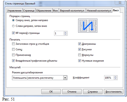
To print, you also need to configure the page settings, that is, paper size, sheet orientation, headers and footers, print direction, etc. Let's do this through the menu item Format > Page and on the tabs of the dialog box the page is configured (Fig. 49, 50, 51). Preview allows you to see how your document will look on paper.

To view the page area, use the menu item View > Page Layout(Fig. 52). By moving the borders (blue) of the page, we change the area of the page for printing by changing the scale, which we will see through Format > Page > Sheet > Scale.

You can save time when creating a SharePoint list by importing a spreadsheet file. When you create a list from a spreadsheet, its column headings become the list, and the remaining data is imported as list items. Importing a spreadsheet is also a way to create a list without a default column header.

Important:

Important: If you receive a message that says that the spreadsheet you want to import is invalid or does not contain data, add the SharePoint site you are using to the list of Trusted Sites tab.

Create a list from a spreadsheet in SharePoint Online 2016 and 2013

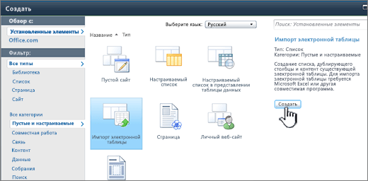
On the site where you want to add the list, click Options and select Add application.

In field Find an app Type "spreadsheet" and click the search icon.

On the search results page, click Import a spreadsheet.
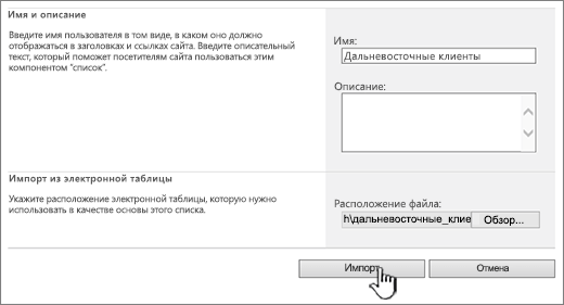
On the page New application enter Name list.
Enter description(not necessary).

The description appears below the name in most views. The description of the list can be changed in its parameters.

Click the button Review to find the spreadsheet, or enter the path to it in the field File location. When finished, press the button Import.

The spreadsheet opens in Excel and a window appears.

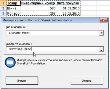
In the window Import to Windows list SharePoint Services select item Table range, Cell range or Named range. If you want to specify the range manually, select Cell range and click Select range. In a spreadsheet, click the top left cell, press and hold SHIFT key and select the bottom right cell of the range.

The range will be indicated in the field Select range. Click the button Import.

List or click the Options button and click List options.

The table data will appear as a list in SharePoint.

Create a list from a spreadsheet in SharePoint 2010 or SharePoint 2007

On the menu Site Actions select team View all site content and press the button Create .

Note: SharePoint sites may look different. If you can't find an element, such as a command, button, or link, contact your administrator.

In SharePoint 2010, under All categories click Blank and customizable, select and press the button Create.

In SharePoint 2007, under Custom Lists select Import Spreadsheet and press the button Create.
Enter a name for the list in the field Name. Field Name is mandatory.

The name appears at the top of the list in most views, becomes part of the web address of the list page, and appears in navigation elements to make it easier to find. The list name can be changed, but the web address will remain the same.

Enter a description of the list in the field Description. Field Description is optional.

The description appears below the name in most views. The list description can be changed.
Click the button Review to select the spreadsheet, or enter its path in the field File location, and then click the button Import.

In the dialog box Import into a Windows SharePoint Services list select Range type and then in the section Select range specify the range in the spreadsheet that you want to use to create the list.

Note: Some spreadsheet editors allow you to select the range of cells you want directly in the spreadsheet. The table range and named range must already be defined in the table to be selected in the dialog box Import into a Windows SharePoint Services list.

Click the button Import.

After importing the spreadsheet, check the list columns to ensure that the data was imported correctly. For example, you might want to specify that a column contains monetary values rather than numbers. To view or change the parameters of the list, open it, go to the tab List or click the Options button and click List options.

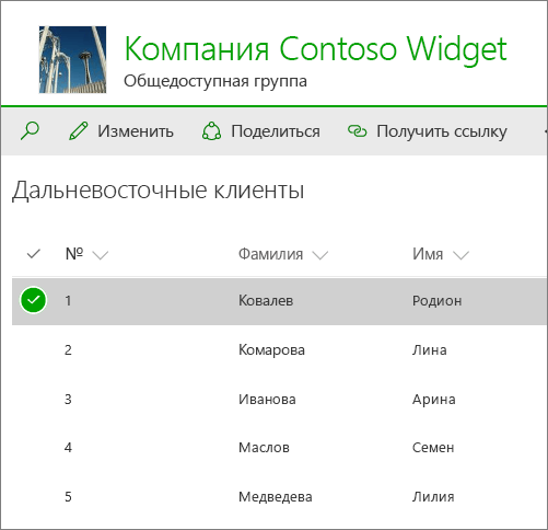
The column types that are created for the list are based on the data types in the spreadsheet columns. For example, a spreadsheet column that contains dates typically becomes a date column in a SharePoint list. The image below shows a SharePoint list that was created by importing the above spreadsheet.

All versions of SharePoint support importing spreadsheets, but the steps involved are slightly different. Excel was used in these examples, but another one will also work compatible editor. If the spreadsheet editor format is not supported, export the data to a comma-separated value (CSV) file and import the file.

For links to articles about setting up an imported list and adding it to a page or site, see Lists Overview.

Note: Typically, columns in a SharePoint site are configured based on the type of data they contain. However, after you import the list, check the columns and data to ensure that the import was completed correctly. For example, you might want to specify that a column contains monetary values rather than numbers. To view or change the options for a list, open it, and then click List options on the menu Options.

Add a site to the trusted sites zone

Open Internet browser Explorer, click the button Service and select Internet Options.

Go to the tab Safety, click the icon Trusted nodes and press the button nodes.

You are on the site will be displayed in Add this website to the zone: fields, click the button Add.

Click the button Close, and then - OK.

Was this article helpful? If yes, please leave your review at the bottom of the page. Otherwise, share your opinion - what needs to be added or made clearer. Please provide your SharePoint version, OS and browser. We will read your review, double-check the information and, if necessary, add and update this article.

Note: Disclaimer regarding machine translation. This article has been translated using computer system without human intervention. Microsoft offers these machine translations to help users who don't know in English, read materials about Microsoft products, services and technologies. Since the article was translated using machine translation, it may contain lexical, syntax and grammatical errors.

Spreadsheets in Microsoft Excel

1. Introduction

2. Creation of electronic Microsoft tables Excel

3. Basic concepts of spreadsheets

4. Entering, editing and formatting data

5. Calculations in spreadsheets

6. Copying cell contents

7. Building charts and graphs

Tables are used to present data in a convenient form. The computer allows you to represent them in electronic form, and this makes it possible not only to display, but also to process data. The class of programs used for this purpose is called spreadsheets.

A special feature of spreadsheets is the ability to use formulas to describe the relationship between the values of different cells. Calculation by given formulas is performed automatically. Changing the contents of a cell leads to the recalculation of the values of all cells that are connected to it by formula relations and, thereby, to updating the entire table in accordance with the changed data.

The use of spreadsheets simplifies working with data and allows you to obtain results without manual calculations or special programming. The most widespread use of spreadsheets is in economic and accounting calculations, but also in scientific and technical tasks, spreadsheets can be used effectively, for example, for:

· Carrying out similar calculations over large sets data;

· automation of final calculations;

· solving problems by selecting parameter values, tabulating formulas;

· processing the results of experiments;

· searching for optimal parameter values;

· preparation spreadsheet documents;

· constructing charts and graphs based on available data.

One of the most common means of working with documents that have a tabular structure is Microsoft program Excel.

Creating Microsoft Excel Spreadsheets

Microsoft Excel is designed to work with data tables, mainly numerical ones. When creating a table, you enter, edit, and format text and numeric data, as well as formulas. The presence of automation tools facilitates these operations. The created table can be printed.

Spreadsheet Basics

An Excel document is called a workbook. A workbook is a collection of worksheets, each of which has a tabular structure and can contain one or more tables. In the document window in Excel, only the current worksheet is displayed, with which you are working. Each worksheet has a title, which appears on the worksheet label that appears at the bottom of the worksheet. Using shortcuts, you can switch to other worksheets included in the same workbook. To rename a worksheet, double-click on its tab.

The worksheet consists of rows and columns. The columns are headed with capital Latin letters and, further, with two-letter combinations. In total, the worksheet can contain up to 256 columns, numbered A through IV. Lines are numbered sequentially, from 1 to 65,536 (the maximum allowed line number).

Cells and their addressing. Table cells are formed at the intersection of columns and rows. They are the minimum elements for storing data. The designation of an individual cell combines the column and row numbers (in that order) at the intersection of which it is located, for example: A1 or DE234. The cell designation (its number) serves as its address. Cell addresses are used when writing formulas that define the relationship between values located in different cells.

One of the cells is always active and is highlighted by the active cell frame. This frame plays the role of a cursor in Excel. Input and editing operations are always performed in the active cell. You can move the frame of the active cell using the cursor keys or the mouse pointer.

If you want to select a rectangular range of cells, you can do this by dragging the pointer from one corner cell to the opposite one diagonally. The frame of the current cell expands to cover the entire selected range. To select an entire column or row, click on the column (row) header. By dragging the pointer over the headings, you can select multiple consecutive columns or rows.

Entering, editing and formatting data

A single cell can contain one of three types of data: text, number, or formula, or remain empty. When saving a workbook, Excel writes to a file only the rectangular area of worksheet adjacent to the upper left corner (cell A1) and containing all filled cells.

The type of data placed in the cell is determined automatically as you enter it. If the data can be interpreted as a number, Excel will do so. Otherwise, the data is treated as text. Entering a formula always begins with the symbol “=” (equal sign).

Entering text and numbers. Data is entered directly into the current cell or into the formula bar located at the top of the program window directly below the toolbars. The input location is marked with a text cursor. If you start typing by pressing the alphanumeric keys, the data in the current cell is replaced with the text you type. If you click on the formula bar or double-click on the current cell, the old contents of the cell are not deleted and you can edit it. The entered data is displayed in any case: both in the cell and in the formula bar.

To complete the entry, saving the entered data, use the Enter button in the formula bar or Enter key. To cancel changes made and restore the cell to its previous value, use the Cancel button in the formula bar or the Esc key. The easiest way to clear the current cell or selected range is to use the Delete key.

Formatting cell contents. By default, text data is aligned to the left edge of the cell, and numbers are aligned to the right. To change the display format of the data in the current cell or selected range, use the Format > Cells command. The tabs of this dialog box allow you to select the format for recording data (the number of decimal places, indicating the monetary unit, how the date is written, etc.), set the direction of the text and the method of its alignment, define the font and style of characters, control the display and appearance of frames, and set the background color.

Spreadsheet calculations

Formulas. Calculations in Excel tables are carried out using formulas. A formula can contain numeric constants, cell references, and Excel functions connected by mathematical symbols. Parentheses allow you to change the standard order of actions. If a cell contains a formula, the worksheet displays the current result of that formula. If you make a cell current, the formula itself is displayed in the formula bar.

The rule for using formulas in Excel is that if the value of a cell actually depends on other cells in the table, you should always use a formula, even if the operation can easily be done in your head. This ensures that subsequent editing of the table will not violate its integrity and the correctness of the calculations performed in it.

Cell references. The formula can contain links, that is, addresses of cells whose contents are used in calculations. This means that the result of the formula depends on the number in another cell. The cell containing the formula is therefore a dependent cell. The value displayed in a formula cell is recalculated when the value of the referenced cell changes.

A cell reference can be specified in different ways. First, the cell address can be entered manually. Another way is to click on the desired cell or select the range whose address you want to enter. The cell or range is highlighted with a dotted frame.

All Excel dialog boxes that require you to specify cell numbers or ranges contain buttons attached to the corresponding fields. When you click this button, the dialog box is minimized to the smallest possible size, making it easier to select the desired cell (range) by clicking or dragging.

Absolute and relative links. By default, cell references in formulas are treated as relative. This means that when you copy a formula, the addresses in the references automatically change according to the relative location of the original cell and the copy being created.

Let, for example, in cell B2 there is a link to cell AZ. In relative view, we can say that the reference points to a cell that is one column to the left and one row below the given one. If the formula is copied to another cell, then this relative reference indication will remain. For example, when you copy a formula into cell EA27, the link will continue to point to the cell to the left and below, in this case cell DZ28.

With absolute addressing, the reference addresses do not change when copied, so the referenced cell is treated as a non-tabular cell. To change the addressing method when editing a formula, select the cell reference and press F4. Cell number elements that use absolute addressing are preceded by a $ character. For example, when pressing the F4 key successively, the cell number A1 will be written as A1, $A$1, A$1 and $A1. In the last two cases, one of the components of the cell number is considered as absolute, and the other as relative.

Copying cell contents

Copying and moving cells in Excel can be done using the drag-and-drop method or via the clipboard. When working with a small number of cells, it is convenient to use the first method; when working with large ranges, it is convenient to use the second.

Drag and drop method. To use drag-and-drop to copy or move the current cell (selected range) along with its contents, move the mouse pointer over the frame of the current cell (it will appear as an arrow). Now the cell can be dragged anywhere on the worksheet (the insertion point is marked with a tooltip).

To select the method of performing this operation, as well as for more reliable control over it, it is recommended to use special drag and drop using the right mouse button. In this case, when you release the mouse button, a special menu appears in which you can select the specific operation to be performed.

Using the clipboard. Transferring information via the clipboard has certain features in Excel related to the complexity of control over this operation. First, you need to select the range to be copied (cut) and give the command to place it on the clipboard: Edit > Copy or Edit > Cut. Pasting data into a worksheet is only possible immediately after it is placed on the clipboard. Attempting to perform any other operation will cancel the copy or move process that was in progress. However, there is no data loss because the “cut” data is removed from its original location only when the insertion occurs.

Finding a solution. This add-in is used to solve optimization problems. Cells for which they are selected optimal values and restrictions are set and selected in the Solution Search dialog box, which is opened using the Tools > Solution Search command.

Data collection template wizard. This add-in is designed to create templates that serve as forms for entering records into a database. When a workbook is created from a template, the data entered in it is automatically copied to the database associated with the template. The wizard is launched using the command Data > Template Wizard.

Web Form Wizard. Add-in Designed to create a form placed on a Web site. The form is organized in such a way that the data entered by visitors is automatically added to the database associated with the form. The Excel form for collecting data must be created on a worksheet in advance. Setting up the data collection system is organized using a wizard, which is launched by the command Tools > Wizard > Web Form.

Building charts and graphs

In Excel, the term chart is used to refer to all types of graphical representation numerical data. Construction graphic image is made on the basis of a series of data. This is the name given to a group of cells with data within a single row or column. You can display multiple data series on one chart.

The diagram is an insert object embedded on one of the sheets of the workbook. It can be located on the same sheet on which the data is located, or on any other sheet (often a chart is set aside to display separate sheet). The chart remains connected to the data on which it is based, and when that data is updated, it immediately changes its appearance.

To create a chart, you usually use the Chart Wizard, launched by clicking the Chart Wizard button on the standard toolbar. It is often convenient to pre-select the area that contains the data that will be displayed in the chart, but you can also specify this information as part of the wizard.

Chart type. At the first stage of the work, the wizard selects the shape of the diagram. Available forms are listed in the Type list on the Standard tab. For the selected chart type, several options for presenting data are indicated on the right (View palette), from which you should select the most suitable one. The Custom tab displays a set of fully formed chart types with ready-made formatting. After specifying the shape of the diagram, click on the Next button.

Data selection. The second stage of the wizard is used to select the data on which the chart will be built. If a data range has been selected in advance, an approximate representation of the future chart will appear in the preview area at the top of the wizard window. If the data forms a single rectangular range, then it is convenient to select them using the tab

Data range. If the data does not form a single group, then information for drawing individual data series is set on the Series tab. The chart preview automatically updates as the data set being displayed changes.

Design of the diagram. The third stage of the wizard (after clicking the Next button) is to select the design of the diagram. On the tabs of the wizard window you can set:

· chart title, axes labels (Titles tab);

· display and marking of coordinate axes (Axes tab);

· displaying a grid of lines parallel to the coordinate axes (Grid Lines tab);

· description of the constructed graphs (Legend tab);

· displaying labels corresponding to individual data elements on the chart (Data Labels tab);

· presentation of the data used to construct the graph in the form of a table (Data Table tab).

Depending on the chart type, some of the tabs listed may not be available.

Chart placement. On last stage The wizard (after clicking the Next button) specifies whether to use a new worksheet or one of the existing ones to place the diagram. Typically this selection is only important for later printing of the document containing the diagram. After clicking the Finish button, the diagram is created automatically and inserted into the specified worksheet.

Editing a diagram. Ready diagram can change. It consists of a set of individual elements, such as the graphs themselves (data series), coordinate axes, chart title, plotting area, etc. When you click on a chart element, it is highlighted with markers, and when you hover the mouse pointer over it, it is described with a tooltip. You can open a dialog box for formatting a chart element through the Format menu (for a selected element) or through context menu(Format command). The various tabs in the dialog box that opens allow you to change the display options for the selected data item.

If you need to make significant changes to the chart, you should use the Chart Wizard again. To do this, open the worksheet with the chart or select a chart embedded in the data worksheet. By launching the Chart Wizard, you can change current parameters, which are considered in the wizard windows as default.

To delete a chart, you can delete the worksheet on which it is located (Edit > Delete Sheet), or select a chart embedded in a worksheet containing data and press Delete.

Introduction.

Spreadsheets is a numerical data processing program that stores and processes data in rectangular tables.

Excel contains many mathematical and statistical functions, thanks to which it can be used by schoolchildren and students to calculate coursework, laboratory work. Excel is heavily used in accounting - in many companies it is the main tool for document preparation, calculations and creating charts. Naturally, it has the corresponding functions. Excel can even act as a database.

If you know how to run at least one Windows program, you know how to run any windows program. It doesn't matter whether you're using Windows 95 or Windows 98 or another Windows.

Most programs are launched the same way - through the Start menu. To launch Excel, do the following:

1. Click the Start button on the taskbar

2. Click the Programs button to open the Programs menu

3. Choose Microsoft Office/Microsoft Office - Microsoft Excel

4. Select Microsoft Office /Microsoft Office - Microsoft Excel

Representing numbers on a computer.

In a computer, all numbers are represented in binary form, that is, as combinations of zeros and ones.

If you allocate 2 bits to represent a number in a computer, then you can represent only four different numbers: 00, 01, 10 and 11. If you allocate 3 bits to represent a number, you can represent 8 different numbers: 000, 001, 010, 011, 100, 101, 110, 111. If you select N bits to represent a number, then you can represent 2n different numbers.

Let 1 byte (8 bits) be used to represent a number. Then you can imagine: 28 = 256 different numbers: from 0000 0000 to 1111 1111. If you translate these numbers into decimal system, it turns out: 000000002=010, 111111112=25510. This means that when using 1 byte to represent a number, you can represent numbers from 0 to 255. But this is if all numbers are considered positive. However, it is necessary to be able to represent negative numbers as well.

In order for a computer to represent both positive and negative numbers, the following rules are used:

1. The most significant (left) bit of the number is signed. If this bit is 0, the number is positive. If it is equal to 1, the number is negative.

2. Numbers are stored in two's complement. For positive numbers additional code matches the binary representation. For negative numbers The complementary code is obtained from the binary representation as follows:

All zeros are replaced by ones, and all ones are replaced by zeros

One is added to the resulting number

These rules are used when it is necessary to determine how a particular number will be represented in computer memory, or when the representation of a number in computer memory is known, but it is necessary to determine what number it is.

Creating a Spreadsheet

1. To create a table, run the File / New command and click on the Blank Workbook icon in the task area.

2. First you need to mark up the table. For example, the Goods Accounting table has seven columns, which we will assign to columns A to G. Next, we need to create the table headings. Then you need to enter general title tables, and then field names. They must be on the same line and follow each other. The heading can be placed in one or two lines, aligned to the center, right, left, bottom or top edge of the cell.

3. To enter the table title, you must place the cursor in cell A2 and enter the table name “Remaining goods in warehouse”

4. Select cells A2:G2 and execute the Format/Cells command, on the Alignment tab, select the center alignment method and check the merge cells checkbox. Click OK.

5. Creating a table header. Enter field names, for example, Warehouse No., Supplier, etc.

6. To arrange the text in the “header” cells in two lines, you need to select this cell and run the Format / Cells command, on the Alignment tab, select the Wrap by words checkbox.

7. Inserting various fonts. Select the text and select the Format/Cells command, Font tab. Set the font typeface, for example, Times New Roman, its size (point) and style.

8. Align the text in the table header (select the text and click the Center button on the formatting toolbar).

9. If necessary, change the width of the columns using the Format / Column / Width command.

10. You can change line heights using the command Format / Line / Height.

11. You can add a border and fill to cells using the Format / Cell command on the Border and View tabs, respectively. Select a cell or cells and on the Border tab, select a line type and use the mouse to specify which part of the selected range it belongs to. On the View tab, select a fill color for the selected cells.

12. Before entering data into the table, you can format the column cells under the table header using the Format/Cells command, Number tab. For example, highlight vertical block cells under the Warehouse # cell and select Format/Cells on the Number tab, highlight Numeric and click OK

the products did not detect them. Microsoft belatedly took steps to mitigate the risk by adding the ability to disable macros entirely and enable macros when opening a document.

Basic concepts.

A spreadsheet consists of columns and rows. Column headings are designated by letters or combinations (FB, Kl, etc.), row headings are designated by numbers.

Cell - intersections of column and row.

Each cell has its own own address, which is made up of a column header and a row. (A1, H3, etc.). The cell on which the actions are performed is highlighted with a frame and is called active.

In Excel, tables are called worksheets, which are made up of cells. ON Excel sheet There may also be headings, captions, and additional data cells with explanatory text.

Worksheet- the main document type used for storing and processing data. While working, you can enter and change data on several sheets at once, named by default Sheet1, Sheet2, etc.

Each spreadsheet file is a workbook consisting of several sheets. In Excel Versions 5.0/7.0, the workbook contains 16 sheets, and in Excel versions 97 and Excel 2000 contains only 3. The number of sheets in the workbook can be changed.

One way to organize work with data in Excel is to use ranges. Cell range is a group of related cells (or even a single related cell) that can include columns, rows, combinations of columns and rows, or even an entire worksheet.

Ranges are used to solve a variety of problems, such as:

1. You can select a range of cells and format them all at once

2. Use a range to print only the selected group of cells

3. Select a range to copy or move data to groups

4. But it is especially convenient to use ranges in formulas. Instead of referring to each cell individually, you can specify the range of cells you want to perform calculations on.

Basic tools.

Button	Description	Button	Description
	Opens new book		Opens the Open Document dialog box
	Saves the file		Sends a file or current sheet via e-mail
	Printing a file		Displays the file in preview mode
	Runs a spell checker		Cuts the selected data to the Clipboard
	Copies the selected data to the Clipboard		Pastes cut or copied data from the Clipboard
	Selects the Format Painter tool		Inserts a hyperlink
	AutoSum function		Sorts data in ascending order
	Sorts data in descending order		Launches the Chart Wizard
	Opens drawing tools		Changes the scale of the image on your sheet
	Changes font size		Makes data bold
	Italicizes data		Emphasizes data
	Align data left, center, and right		Centers data in selected cells
	Applies currency format		Applies percentage format
	Applies comma formatting		Increases the number after the decimal point
	Reduces the number of decimal places		Adds a border
	Paints the background with the selected color		Changes the font type
	Changes text color

Data types and format.

Basic data types.

When working with spreadsheets, there are three main types of data: number, text And formula.

Numbers in electronic Excel tables can be written in regular numeric or exponential format, such as 195.2 or 1.952E+02. By default, numbers are aligned to the right in a cell. This is explained by the fact that when placing numbers under each other, it is convenient to have alignment by digits (units under units, tens under tens, etc.)

By text is a sequence of characters consisting of letters, numbers and spaces, for example the entry “45 bits” is text. By default, text is aligned left in a cell.

Formula must begin with an equal sign and can include numbers, cell names, functions, and mathematical operations signs. But the formula cannot include text. For example, the formula =A1+B1 provides the addition of numbers stored in cells A1 and B1, and the formula =C3*9 multiplies the number stored in cells C3 by 9.

For example =A1+B2. When you enter a formula in a cell, it is not the formula itself that is displayed, but the result of calculations using this formula. If the original values included in the formula change, the result is recalculated immediately.

Data format.

There is a need to apply various formats data presentation.

The default is a number format that displays two decimal places.

Exponential format is used when a number containing a large number of digits does not fit in the cell (for example, 3500000000, then it will be written in 5.00E+09).

Since Excel is designed to process numbers, it plays an important role correct setting their format. For humans, the number 10 is simply one and zero. From Excel's point of view, these two numbers can be completely various information depending on whether it denotes the number of employees of the company, a monetary value, a percentage of the whole or a fragment of the "Top 10 Firms" title. In all four situations, this number should be displayed and processed differently. Excel supports following formats:

General - assigned automatically if the format is not specifically specified.

Number - the most common way to represent numbers

Currency - monetary values

Financial (Accounting) - monetary values aligned by the separator of the integer and fractional part

Date - date or date and time

Time - time or date and time

Percentage - cell value multiplied by 100 with a % symbol at the end

Fraction - rational fractions with numerator and denominator

Exponential (Scientific) - decimal fractional numbers

Text - text data is displayed in the same way as strings are entered and processed, regardless of their content

Additional (Special) - formats for working with databases and address lists

Custom - user-configurable format

Selecting a Data Format

1. Enter the Format-Cell command

2. In the Format Cells dialog box, select the Number tab.

3. In the Number formats list: select the most appropriate format.

The Alignment tab is defined:

1. Alignment - a way to align data in a cell horizontally (left or right, by value, centered, centered, justified, filled) or vertically (bottom or top,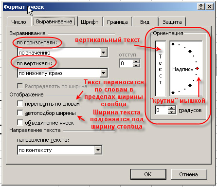

center or height);

2. Display - determines whether text can be transferred in a cell, according to words, allows or prohibits merging cells, sets automatic selection of cell widths.

3. Text orientation

Font tab - changes the font, style, size, color, underline and text effect in selected cells;

Border tab - creates a frame (frame) around the selected block of cells;

View tab - allows you to set the cell shading (color and pattern);

Protection tab - controls hiding formulas and locking cells (prohibiting editing of cell data). You can set protection at any time, but it will only take effect after the sheet or workbook has been protected using the Tools/Protect Sheet command.

Entering a formula

You can enter a formula in two ways. You can enter a formula directly into a cell or use the formula bar. To enter a formula into a cell, do the following actions:

1. Select the cell where you want to enter the formula and start writing with the “=” sign. This tells Excel that you are about to enter a formula.

2. Select the first cell or range you want to include in the formula. The address of the cell you reference appears in the active cell and in the formula bar.

3. Enter an operator, such as the "+" sign.

4. Click the next cell or range that you want to include in the formula. Continue entering operators and selecting cells until the formula is complete.

5. When you have finished entering the formula, click the Enter button in the formula bar or press Enter on the keyboard.

6. The cell now shows the result of the calculation. To see the formula, select the cell again. The formula appears in the formula bar.

Another way to enter formulas is to use the Formula Bar. First, select the cell in which you want to enter the formula, and then click the Edit Formula button (the button with equal signs) in the formula bar. The Formula Bar window will appear. The equal sign will be automatically entered before the formula. Start typing the cells you want to use in the formula and the operators needed to perform the calculation. After you enter the entire formula, click the OK button. The formula will appear in the formula bar, and the calculation result will appear in the worksheet cell.

Often you need to use the Function Wizard to create a formula.

Functions can be entered manually, but Excel provides a function wizard that allows you to enter them semi-automatically and with virtually no errors. To call the Function Wizard, click the Insert Function button on the standard toolbar, execute the Insert/Function command, or use the keyboard shortcut. The Function Wizard dialog box will then appear, allowing you to select the desired function.

The window consists of two interconnected lists: Category and Function. When you select one of the elements of the Category list in the Function list, the corresponding list of functions appears.

When you select a function, a brief description of it appears at the bottom of the dialog box. When you click the ok button, you go to next step. Step2.

Functions in Excel

To speed up and simplify computing Excel work puts at the user's disposal a powerful apparatus of worksheet functions that allow almost all possible calculations to be carried out.

In total, MS Excel contains more than 400 worksheet functions (built-in functions). All of them, according to their purpose, are divided into 11 groups (categories):

1. financial functions;

2. date and time functions;

3. arithmetic and trigonometric (mathematical) functions;

4. statistical functions;

5. functions of links and substitutions;

6. database functions (list analysis);

7. text functions;

8. logical functions;

9. information functions(checking properties and values);

10. engineering functions;

11. external functions.

Task II