Relative and absolute cell addresses. Working with cells. Filling and formatting
This program can be used for the following purposes:
· Accounting. The program has quite powerful functions for calculating financial and accounting statements.
· Budgeting. In this program you can create different kinds budget for business and personal needs, for example, you can create a marketing budget plan.
· Reports. This program can create reports to analyze and summarize data, such as reports that measure the effectiveness of a project.
· Planning. The program is an excellent tool for creating professional plans.
· Use of calendars. The program's workspace is designed as a grid, so it can be used to create different types of calendars, such as a fiscal year calendar for Tracking business events and business highlights.
The program window consists of:
· The tab bar (ribbon), which is located at the top of the program window. Located on the tape certain sets commands (program functions), which are grouped into commands and groups (by default, a ribbon containing 7 tabs is displayed; when the program starts, the “Home” tab is active). When moving to new work objects (formula diagrams), new tabs appear.
· Above the tab bar is the quick access, which includes the most used commands (by default, the panel contains a button to save data, cancel and repeat the action). To the right is an icon, by clicking on it with the left mouse button, you can open a list of additional tasks. There you can select the buttons that will be displayed on the Quick Access Toolbar.
![]()
· Below the tab strip there is a name bar and a formula bar. The name bar will display the name active object or cells, and the formula bar will display the formula of the active cell.
Name string.
Formula bar.
· The main part of the window is occupied by the working area.
· In the lower right window of the program there are commands that serve for the most advantageous viewing of the document.

Book in Excel 2010
The book consists of:
3 sheets is the standard, maximum 255 sheets. Each sheet consists of cells that are formed by the intersection of rows and columns. The rows are numbered in Arabic numerals (1,2,3), and the columns in capital English letters (A, B, C).
Editing tables in Excel 2010
In order to change the column width or row height, you need to insert the row names between the letters with the column names or numbers and drag them in the desired direction.
To set a rule for filling cells, you need to enter data in 2 adjacent cells, select them and, using the fill marker, which is located in the lower right corner, drag it to the required amount.
Creating formulas in Excel 2010
The formula begins with the “=” sign, cell addresses are written only to English language. In order not to write down the cell address, you can simply select it with the left mouse button when writing a formula.


How to build a function in Excel 2010 (how to do calculations in Excel 2010)
Program Microsoft Excel convenient for drawing up tables and making calculations. A workspace is a set of cells that can be filled with data. Subsequently - format, use for building graphs, charts, summary reports.
Working in Excel with tables for novice users may seem difficult at first glance. It differs significantly from the principles of creating tables in Word. But we'll start small: by creating and formatting a table. And at the end of the article you will already understand that the best tool for creating tables you can't beat Excel.
How to Create a Table in Excel for Dummies
Working with tables in Excel for dummies is not rushed. You can create a table different ways and for specific purposes, each method has its own advantages. Therefore, first let’s visually assess the situation.
Look carefully at the spreadsheet worksheet:
This is a set of cells in columns and rows. Essentially a table. The columns are labeled with Latin letters. Lines are numbers. If we print this sheet, we get blank page. Without any boundaries.
First let's learn how to work with cells, rows and columns.
How to select a column and row
To select the entire column, click on its name (Latin letter) with the left mouse button.

To select a line, use the line name (by number).

To select several columns or rows, left-click on the name, hold and drag.
To select a column using hot keys, place the cursor in any cell of the desired column - press Ctrl + spacebar. To select a line – Shift + spacebar.
How to change cell borders
If the information does not fit when filling out the table, you need to change the cell borders:


To change the width of columns and height of rows at once in a certain range, select an area, increase 1 column/row (move manually) - the size of all selected columns and rows will automatically change.

Note. To return to the previous size, you can click the “Cancel” button or the hotkey combination CTRL+Z. But it works when you do it right away. Later it won't help.
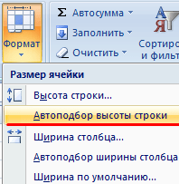
To return the lines to their original boundaries, open the tool menu: “Home” - “Format” and select “Auto-fit line height”
This method is not relevant for columns. Click “Format” - “Default Width”. Let's remember this number. Select any cell in the column whose borders need to be “returned”. Again “Format” - “Column Width” - enter specified by the program indicator (usually 8.43 - the number of characters in the Calibri font with a size of 11 points). OK.
How to insert a column or row
Select the column/row to the right/below the place where you want to insert the new range. That is, the column will appear to the left of the selected cell. And the line is higher.

Right-click and select “Insert” from the drop-down menu (or press the hotkey combination CTRL+SHIFT+"=").

Mark the “column” and click OK.
Advice. For quick insert column, you need to select the column in the desired location and press CTRL+SHIFT+"=".
All these skills will come in handy when creating a table in Excel. We will have to expand the boundaries, add rows/columns as we work.
Step-by-step creation of a table with formulas


Column and row borders will now be visible when printing.

You can format data using the Font menu Excel tables, as in Word.

Change, for example, the font size, make the header “bold”. You can center the text, assign hyphens, etc.
How to create a table in Excel: step-by-step instructions
The simplest way to create tables is already known. But Excel has more convenient option(in terms of subsequent formatting, working with data).
Let's make a “smart” (dynamic) table:

Note. You can take a different path - first select a range of cells, and then click the “Table” button.

Now enter the required information in finished frame. If you need an additional column, place the cursor in the cell designated for the name. Enter the name and press ENTER. The range will automatically expand.

If you need to increase the number of lines, hook it in the lower right corner to the autofill marker and drag it down.
How to work with a table in Excel
With the release of new versions of the program, working with tables in Excel has become more interesting and dynamic. When a smart table is formed on a sheet, it becomes accessible tool“Working with tables” - “Designer”.
Here we can give the table a name and change its size.
Various styles are available, the ability to convert the table into a regular range or a summary report.
Dynamic capabilities spreadsheets MS Excel huge. Let's start with basic data entry and autofill skills:


If we click on the arrow to the right of each subheading, we will get access to additional tools for working with table data.

Sometimes the user has to work with huge tables. To see the results, you need to scroll through more than one thousand lines. Deleting rows is not an option (the data will be needed later). But you can hide it. For this purpose, use numerical filters (picture above). Uncheck the boxes next to the values that should be hidden.
Program Microsoft Office Excel is a table editor in which it is convenient to work with them in every possible way. Here you can also set formulas for elementary and complex calculations, create graphs and diagrams, program, creating real platforms for organizations, simplifying the work of the accountant, secretary and other departments dealing with databases.
How to learn to work in excel on your own
The excel 2010 tutorial describes in detail the program interface and all the features available to it. To start working independently in Excel, you need to navigate the program interface, understand the taskbar, where commands and tools are located. To do this, you need to watch a lesson on this topic.
At the very top of Excel we see a ribbon of tabs with thematic sets of commands. If you move the mouse cursor over each of them, a tooltip appears detailing the direction of action.
Under the ribbon of tabs there is a line “Name”, where the name is written active element and the “Formula Bar,” which displays formulas or text. When performing calculations, the “Name” line is converted into a drop-down list with a default set of functions. You just need to select the required option.
Most of the excel window is occupied by the work area, where tables, graphs are actually built, and calculations are made. . Here the user performs any necessary actions, using commands from the tab ribbon.
At the bottom of excel on the left side you can switch between workspaces. Additional sheets are added here if it is necessary to create different documents in one file. In the lower right corner there are commands responsible for convenient viewing created document. You can select the viewing mode workbook, by clicking on one of the three icons, and also change the scale of the document by changing the position of the slider.
Basic Concepts
The first thing we see when opening the program is Blank sheet, divided into cells representing the intersection of columns and rows. The columns are designated by Latin letters, and the rows by numbers. It is with their help that tables of any complexity are created and the necessary calculations are carried out in them.
Any video lesson on the Internet describes creating tables in Excel 2010 in two ways:

To work with tables, several types of data are used, the main of which are:
- text,
- numerical,
- formula.
By default, text data is aligned to the left of cells, and numeric and formula data is aligned to the right.
To enter the required formula In a cell, you must start with an equal sign, and then by clicking on the cells and putting the required signs between the values in them, we get the answer. You can also use the drop-down list with functions located in the upper left corner. They are recorded in the “Formula Bar”. It can be viewed by making a cell with a similar calculation active.
VBA to excel
 The programming language built into the application allows you to simplify work with complex data sets or repetitive functions in Excel. Visual Basic for Applications (VBA). Programming instructions can be downloaded on the Internet for free.
At Microsoft Office Excel 2010 VBA is disabled by default. In order to enable it, you need to select “Options” in the “File” tab on the left panel. In the dialog box that appears, on the left, click “Customize Ribbon”, and then on the right side of the window, check the box next to “Developer” so that such a tab appears in Excel.
When starting to program, you need to understand that an object in Excel is a sheet, workbook, cell and range. They obey each other, so they are in a hierarchy.
Application plays a leading role . Next come Workbooks, Worksheets, Range. Thus, you need to specify the entire hierarchy path to access a specific cell.
Another important concept is properties. These are the characteristics of objects. For Range it is Value or Formula.
The methods are certain commands. They are separated from the object by a dot in VBA code. Often when programming in Excel, the Cells (1,1) command is needed. Select. In other words, you need to select a cell with coordinates (1,1), that is, A 1.
The Excel application is included in the standard Microsoft Office 2010 package and is used for PC users to work with spreadsheets.
I'll try to answer the question about how to work in Excel. With this program we first of all create Excel workbook, consisting of several sheets. It can be created in two ways.
On the PC desktop, right-click in context menu select: "create Microsoft Sheet Excel" or "open the program using the shortcut and create a new workbook."
Excel allows you to perform data analysis, tables and summary reports, and make various mathematical calculations in a document by entering formulas, build professional charts and graphs that allow you to analyze table data.
It is not so easy to briefly talk in a short article about how to work in Excel, what are the areas of application of the program, and what formulas are needed for. But let's start in order.
There is a book open in front of you that contains empty cells. Before you start working with them, study them carefully depending on the version. The 2010 version has a tab ribbon at the top. The first of them is “Main”. Next are the tabs for performing user tasks: “Insert”, “Page Layout”, “Formulas”, “Data”, “Review”, “View” and “Add-Ins”. It is necessary to carefully familiarize yourself with the tools located in these tabs.

Notice the Office button. It is intended for calling commands and is located in the program window, at the top left.
Let's say we create a financial document where we can see the movement Money, income data, profit and loss calculation. Here it is possible to perform a complete analysis of financial activities. How to work in Excel to create such a document?
First, we enter digital data into the cells, which we combine into a table. To enter data into a cell, you must make it active. To do this, select it with a mouse click and enter the required information.
After filling out the entire field, we design the table by selecting the entire work area. In the right-click menu, select the “Cell Format” line. Here we select the "Borders" tool and apply it.

This menu also provides other commands for editing tables. The reference book will teach you how to work in Excel. Check them out for yourself. Purchase and carefully study the tutorial, which details the principles of how to work in Excel 2010. Choose a reference book with tasks, since theory without practice is ineffective. By completing assignments, you will be able to consolidate your theoretical knowledge and quickly master the principles of working in Excel.
Working with formulasExcel
After preparing the tables for performing calculations in automatic mode(A Excel program, in fact, is intended for this), you need to enter the necessary numbers and signs into the formula bar and into the cell itself. Working with formulas in Excel is one of the advantages of spreadsheets. Here you can perform any operations: addition, subtraction, multiplication, division, extraction square roots, calculation of functions and logarithms; You can find the sum of numbers and the arithmetic mean.
The formula is preceded by an equal sign, which is placed in the formula bar, and then in parentheses function arguments are written, separated from each other by a semicolon.
For a more in-depth study of the principles of work in this program, you need to take special courses. To begin with, all you need is a desire to learn the rules that will allow you to learn how to work in Excel.
Which allow you to optimize work in MS Excel. And today we want to bring to your attention a new portion of tips for speeding up actions in this program. Nikolai Pavlov, the author of the “Planet Excel” project, will talk about them, changing people’s understanding of what can actually be done using this wonderful program and everything Office package. Nikolay is an IT trainer, developer and expert in Microsoft products Office, Microsoft Office Master, Microsoft Most Valuable Professional. Here are the techniques he personally tested for accelerated work in Excel. ↓
Quickly add new data to a chart
If for your already constructed chart there is new data on the sheet that needs to be added, then you can simply select the range with new information, copy it (Ctrl + C) and then paste it directly into the diagram (Ctrl + V).
This feature only appeared in the latest Excel versions 2013, but worth upgrading to new version ahead of schedule. Let's assume that you have a list of full names (Ivanov Ivan Ivanovich), which you need to turn into abbreviated names (Ivanov I.I.). To perform this conversion, you just need to start writing the desired text in the adjacent column manually. On the second or third Excel line will try to predict our actions and perform further processing automatically. All you have to do is click Enter key to confirm and all names will be converted instantly.

In a similar way, you can extract names from emails, merge full names from fragments, etc.
Copying without breaking formats
You most likely know about the “magic” autofill marker - a thin black cross in the lower right corner of a cell, by pulling which you can copy the contents of the cell or a formula to several cells at once. However, there is one unpleasant nuance: such copying often violates the design of the table, since not only the formula is copied, but also the cell format. This can be avoided if, immediately after drawing a black cross, click on the smart tag - special icon appears in the lower right corner of the copied area.
If you select the “Copy values only” option (Fill Without Formatting), then Microsoft Excel will copy your formula without formatting and will not spoil the design.

IN latest version Excel 2013 now has the ability to quickly display interactive map your geodata, for example sales by city, etc. To do this, go to the “App Store” (Office Store) on the “Insert” tab and install the plugin from there Bing Maps. This can also be done via a direct link from the site by clicking the Add button. After adding a module, you can select it from the My Apps drop-down list on the Insert tab and place it on your worksheet. All you have to do is select your data cells and click on the Show Locations button in the map module to see our data on it.

If desired, in the plugin settings you can select the type of chart and colors to display.
If the number of worksheets in your book exceeds 10, then it becomes difficult to navigate through them. Right-click on any of the sheet tab scroll buttons in the lower left corner of the screen.

Have you ever matched the input values in your Excel calculation to get the output desired result? At such moments you feel like a seasoned artilleryman, right? Just a couple of dozen iterations of “undershooting - overshooting”, and here it is, the long-awaited “hit”!
Microsoft Excel can do this adjustment for you, faster and more accurately. To do this, click the “What If Analysis” button on the “Insert” tab and select the “Parameter Selection” command (Insert - What If Analysis - Goal Seek). In the window that appears, specify the cell where you want to select the desired value, the desired result and the input cell that should change. After clicking “OK,” Excel will perform up to 100 “shots” to find the total you require with an accuracy of 0.001.

If this detailed review didn't cover everything useful tips MS Excel that you know about, share them in the comments!


