How to make comparisons in excel. Comparing data in Excel on different sheets.
Inquire add-in for Excel 2013 allows you to compare and analyze Excel documents for connections between them, the presence of erroneous formulas and identifying differences between .xlsx files. Let's look at the moments when this add-in may be useful to you and how to use it.
Launching the Inquire add-in
The Inquire add-in for Excel comes bundled with standard set Excel 2013 and no additional installation packages are required. Just enable it in add-ons. More early versions Excel does not support this add-in. In addition, at the time of writing, the add-on was only available in English.
To launch Inquire, go to the tab File –> Options. In the dialog box that appears, select the tab Add-ons, in the dropdown menu Control select Add-onsCOM and click the button Go. A window will appear Add-ons for the component object model (COM), where you will need to check the box Inquire and press the button OK.

After launching the add-in, the ribbon will display new inset Inquire.
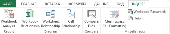
Let's see what benefits this add-on gives us.
Workbook Analysis
Analysis workbook used to identify workbook structure, formulas, errors, hidden sheets, etc. To use this tool, go to the group Report and click the button Workbook Analysis. The result of the add-in is presented below.
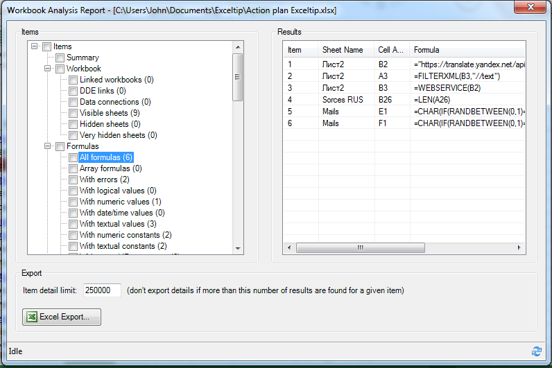
Surely many people paid attention to the point Veryhiddensheets(Very hidden sheets). This is not a joke, in Excel you can actually hide a worksheet “well” using the VisualBasic editor. We will talk more about this in our subsequent articles.
Linking to Worksheets
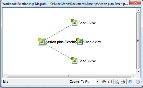
In Group Diagram, There are three tools for defining connections between workbooks, sheets and cells. They allow you to indicate relationships between Excel elements. This functionality can be useful when you have a large number of cells with links to other books. Trying to unravel this tangle can take a significant amount of time, while the Inquire add-in allows you to visualize data dependencies.
To build a dependency diagram, in the group Diagram select one of the items WorkbookRelationship, WorksheetRelationship or CellRelationship. The choice will depend on what kind of dependency you want to see: between workbooks, sheets or cells.
In the picture below you will see the workbook relationship diagram that Excel produced when I clicked the button WorkbookRelationship.
Comparing two files
The next Inquire add-in tool for Excel is Compare– allows you to compare two files cell by cell and point out any differences between them. This tool may be needed when you have multiple revisions of the same file and need to understand what changes have been made to the latest versions.
To use this tool you will need two files. In Group Compare choose CompareFiles. In the dialog box that appears, we must select the files that we want to compare and click the button Compare.
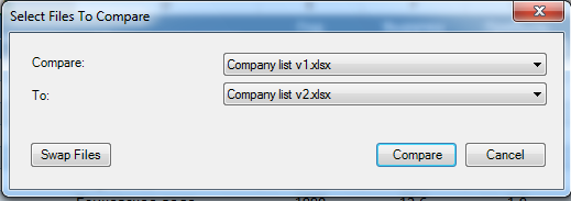
In our case, it's two identical files, to one of which I deliberately made some changes.
After some deliberation, Excel will produce the result of the comparison, where the differences between the two tables will be indicated in color. In this case, the cell color will be different depending on the type of cell difference (differences can be generated due to values, formulas, calculations, etc.).
![]()
Cleaning up unnecessary formatting
This tool allows you to clear unnecessary formatting from cells in a workbook, such as cells that are formatted but do not contain values. Tool Clean Excess Cell Formatting will help “amateurs” to fill the entire line of a workbook with color, instead of filling certain lines tables.
Every month, the HR person receives a list of employees along with their salaries. It copies the list to new leaf working Excel workbooks. The task is as follows: compare employee salaries, which have changed compared to the previous month. To do this, you need to compare data in Excel using different sheets. Let's use conditional formatting. This way we will not only automatically find all the differences in cell values, but also highlight them with color.
Comparing two sheets in Excel
A company may have more than a hundred employees, some of whom quit, others get jobs, others go on vacation or sick leave, etc. As a result, it may be difficult to compare salary data. For example, the last names of employees will always be in different sequences. How to make a comparison between two Excel tables on different sheets?
Solve this not an easy task Conditional formatting will help us. For example, let's take data for February and March, as shown in the figure:
To find changes on pay slips:
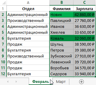
After entering all the conditions for Excel formatting automatically highlighted in color those employees whose salaries have changed compared to the previous month.
The principle of comparing two data ranges in Excel on different sheets:
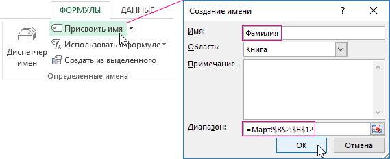
In certain conditions, the MATCH function is essential. Its first argument contains a pair of values that should be found in the source sheet of the next month, that is, "March". A browseable range is defined as a pair of range values defined by names. In this way, strings are compared based on two characteristics: last name and salary. For matches found, a number is returned, which is essentially true for Excel. Therefore, you should use the =NOT() function, which allows you to replace the TRUE value with FALSE. Otherwise, formatting will be applied to cells whose values match. For each pair of values that is not found (that is, a mismatch) &B2&$C2 in the range LastName&Salary, the MATCH function returns an error. The error value is not a boolean value. Therefore, we use the IFERROR function, which will assign a logical value for each error - TRUE. This facilitates the assignment of a new format only for cells without matching salary values in relation to the next month - March.
Sometimes there is a need to compare two MS Excel files. This may be finding discrepancies in prices for certain items or changing any indications, it doesn’t matter, the main thing is that it is necessary to find certain discrepancies.
It would not be amiss to mention that if there are a couple of records in the MS Excel file, then there is no point in resorting to automation. If the file contains several hundred or even thousands of records, then without help computing power A computer is indispensable.
Let's simulate a situation where two files have the same number of lines, and the discrepancy must be looked for in a specific column or in several columns. This situation is possible, for example, if you need to compare the price of goods according to two price lists, or compare the measurements of athletes before and after the training season, although for such automation there must be a lot of them.
As a working example, let's take a file with the performance of fictitious participants: 100-meter run, 3000-meter run, and pull-ups. The first file is a measurement at the beginning of the season, and the second is the end of the season.
The first way to solve the problem. The solution is only using MS Excel formulas.
Since the records are arranged vertically (the most logical arrangement), it is necessary to use the function. If you use horizontal placement of records, you will have to use the function.
To compare 100 meter running performance, the formula is as follows:
IF(VLOOKUP($B2,Sheet2!$B$2:$F$13,3,TRUE)<>D2;D2-VLOOKUP($B2;Sheet2!$B$2:$F$13,3,TRUE);"No difference")
If there is no difference, a message is displayed that there is no difference; if there is a difference, then the value at the end of the season is subtracted from the value at the beginning of the season.
The formula for the 3000 meter run is as follows:
IF(VLOOKUP($B2,Sheet2!$B$2:$F$13,4,TRUE)<>E2;"There is a difference";"There is no difference")
If the final and initial values are not equal, a corresponding message is displayed. The formula for pull-ups can be similar to any of the previous ones; there is no point in giving it additionally. Final file with the discrepancies found is given below.
A little clarification. To make the formulas easier to read, the data from the two files was moved into one (on different sheets), but this could not have been done.
Video comparing two MS Excel files using and functions.
The second way to solve the problem. Solution using MS Access.

This problem can be solved if you first import MS Excel files into Access. As for the method of importing external data itself, there is no difference in finding different fields (any of the presented options will do).
The latter represents the connection Excel files and Access, so when you change data in Excel files, discrepancies will be found automatically when you run a query in MS Access.
The next step after importing is to create relationships between tables. As a connecting field, select the unique field “Item No.”
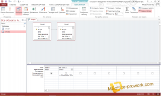
The third step is to create a simple select query using the Query Builder.
In the first column we indicate which records need to be displayed, and in the second - under what conditions the records will be displayed. Naturally, for the second and third fields the actions will be similar.
Video comparing MS files to Excel using MS Access.
As a result of the manipulations performed, all records are displayed, with different data in the field: “Running 100 meters”. The MS Access file is presented below (unfortunately, SkyDrive does not allow embedding as an Excel file)
These two methods exist for finding discrepancies in MS Excel tables. Each has both advantages and disadvantages. Obviously, this is not an exhaustive list of comparisons between the two Excel files. We are waiting for your suggestions in the comments.

Msofficeprowork
Zdevl
Msofficeprowork
Zdevl
I tried it, same thing
Zdevl
I did this before, everything was fine. The Excel version did not change, only the Windows version changed
Msofficeprowork
I understand, then I won’t even give you a hint, I went through the settings, I don’t think I’ve seen a ban on external links. Is it possible to try on another computer? Or tell me, maybe there is a problem in the file (the filter blinks or something else).
Zdevl
Hello.
I have the same problem, I'm trying to select a range in the second file, but nothing is selected. All values are added to the function only from the first file, and it simply does not see the second. Maybe there is something to be enabled in the Excel settings itself?
Good afternoon
This article is devoted to solving this issue, How compare two tables in Excel, or at least two columns. Yes, working with tables is convenient and good, but when you need to compare them, it is quite difficult to do this visually. Maybe you can visually sort a table up to a dozen or two, but when they exceed thousands, then you will need additional tools analysis.
Alas, there is no magic wand with which everything will be done in one click and the information will be verified; it is necessary to prepare data, and write down formulas and other procedures that allow compare two tables in Excel.
Let's consider several options and possibilities compare two tables in Excel:
The easy way
This is the simplest and most basic way How compare two tables in Excel. It is possible to compare both numeric and text values in this way. For example, let's compare two ranges numerical values, in total having written in the next cell the formula for their equality =C2=E2 , as a result, if the cells are equal, we get the answer "TRUE", and if there are no matches, there will be "LIE". Now simple car by copying we copy our formula to the entire range, allowingcompare two tables in Exceland we see the difference.

Quickly highlight values that are different
This is also not a very cumbersome method. If you just need to find and make sure that there are, or are not, differences between the tables, you need to go to the “Home” tab, select the “Find and Select” menu button, having previously selected the range where you need compare two tables in Excel. In the menu that opens, select “Select a group of cells...”
and in the dialog box that appears select "differences by line".


Compare two tables in Excel using conditional formatting
Very good way, in which you can see the value highlighted in color, which when compare two tables in Excel are different. You can apply on the tab "Home" by pressing the button "Conditional Formatting" and select from the list provided "Rule Management". In the dialog box "Conditional Formatting Rules Manager", press the button "Create Rule" and in a new dialog box "Create a formatting rule", select a rule
. In field "Change rule description"
enter the formula =$C2<>$E2 to determine the cell that needs to be formatted and press the button "Format".
In the dialog box "Conditional Formatting Rules Manager", press the button "Create Rule" and in a new dialog box "Create a formatting rule", select a rule
. In field "Change rule description"
enter the formula =$C2<>$E2 to determine the cell that needs to be formatted and press the button "Format".
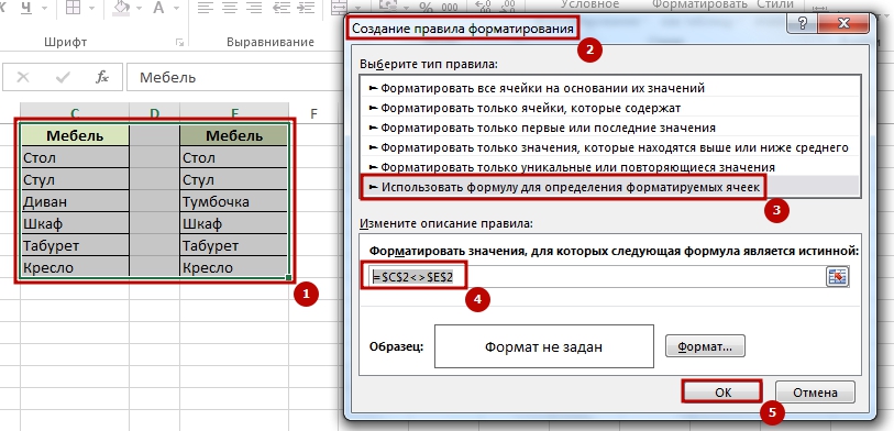 We determine the style of how our value that meets the criterion will be formatted.
 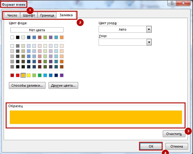 Now our newly created rule has appeared in the list of rules, you select it, click "OK".
And the whole rule applied to our range where we try compare two tables in Excel, and the differences became visible, to which conditional formatting was applied.

How to compare two tables in Excel using the COUNTIF function and rules
All of the above methods are good for ordered tables, but when the data is not ordered, other methods are needed, one of which we will now consider. Let's imagine, for example, we have 2 tables, the values in which are slightly different and we need compare two tables in Excel to determine the value that is different. Select the value in the range of the first table and on the tab "Home", menu item "Conditional Formatting" and click on the item in the list "Create a rule...", select a rule "Use a formula to determine which cells to format", enter the formula= ($C$1:$C$7;C1)=0and select the conditional formatting format. The formula checks the value from specific cell C1 and compares it with the specified range $C$1:$C$7 from the second column. We copy the rule to the entire range in which we compare tables and get values highlighted in the cells that do not repeat.
How to compare two tables in Excel using the VLOOKUP function
In this option we will use , which will allow us compare two tables for coincidences. To compare two bars, enter the formula =VLOOKUP(C2,$D$2:$D$7,1,0) and copy it to the entire range being compared. This formula sequentially begins to check whether there are repetitions of the value from column A in column B, and accordingly returns the value of the element, if it was found there, if the value is not found, we get .

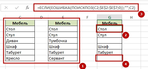
How to compare two tables in Excel IF functions
This option involves the use of a logical one, and the difference between this method is that to compare two columns, not the entire column will be used, but only that part of it that is needed for comparison.
For example, compare two columns A and B on the worksheet, in the adjacent column C we enter the formula: =IF( (MATCH(C2,$E$2:$E$7,0));"";C2) and copy it to the entire . This formula allows you to view consistently whether there are certain elements from the specified column A in column B and returns the value if it was found in column B.