How to increase size in Excel. Excel - preparation for printing and options for printing a document

You already know how to post Excel cells numerical data, perform calculations and present the results in the form of charts. All that remains is to learn how to print received documents. The lesson covers following operations helping to prepare Excel sheets for printing:

page orientation;

Setting up fields;

Adding headers and footers;

Data sorting;

Filtration;

Display row and column headings on all pages;

Hiding cells and sheets;

Pagination.

To quickly print an Excel sheet, just click the Print button on the Standard toolbar. However, the result of this operation will most likely not satisfy you. It is good for outputting drafts, but is completely unsuitable for printing final documents, which must be well designed and do not tolerate the presence of unnecessary information. Therefore, before finally printing Excel sheets, you need to adjust the scale and margins of the pages, sort the table data, select the range of cells to be printed, specify the way tables and charts will be arranged, and perform some other operations.

Page layout

In general, setting print options in Excel is similar to a similar operation in Word. But Excel sheets have their own specifics. It is convenient for the tabular data of the sheet to fit on one page, so adjusting the print scale is required. Wide sheets are usually displayed in landscape orientation, and long tables in portrait orientation. If in Word options Pages, as a rule, are assigned to the entire document at once, but in Excel they are configured separately for each sheet.

Exercise 1: Page orientation and scale

Let's continue working with the Spreadsheet.x1s file and print some of its sheets. In this exercise, you perform the first stage of preparation for printing - setting the page orientation and scale of the output sheet.

Open the file Spreadsheet.xls.

Expand the Formula sheet by clicking on its spine.

The table in this worksheet only has columns for the first six months. Let's expand the table so that it contains data for all 12 months of the year. This will allow you to learn how to print wide tables that do not fit onto the entire sheet.

Select cells B1:G14 and press Ctrl+C to copy them to the clipboard.

Select Insert > Copied Cells to duplicate the cells selected in step 3.

In the dialog box that opens, select the Shift Cells Right radio button, and then click OK. The cells selected in step 3 will be duplicated with new columns added.

Now you need to adjust the column headings. To do this, click on cell B1 and drag the lower left corner of the frame to the right so that the frame covers the range B1:M1. Excel will automatically generate a sequence of month names.

There are empty cells left in column G. To fill them in with the corresponding formulas for calculating sales growth, select the group F10:Fl4, copyit, click on cell G10 right click mouse and select Paste. The shade sheet will look like shown in Fig. 12.1.

Rice. 12.1.Updated Formula Sheet

Select File > Print Setup.

Expand the Page tab in the dialog box that opens, shown in Fig. 12.2.

Rice. 12.2.Setting page orientation and scale

Rice. 12.3.Table at 100% scale

Select the Landscape switch position.

To see the expected placement of numbers on the page, click the Print Preview button. If selected standard size A4 size paper, it turns out that all the columns do not fit on the page (Fig. 12.3).

Press the Page Down key and you will see that the cells in the rightmost column are moved to the second page. It is not comfortable. You should change the scale so that all the width of the table columns fits on one page.

Note

In the resulting table the data columns H-L repeat numbers columns B-G. If you want, change the values ​​in some cells. In the exercises of this lesson specific numeric values cells are unimportant.

Click the Setup button on the toolbar to return to the Page Setup dialog box.

The Scaling section of this dialog box allows you to reduce or enlarge printed objects. Using the Adjust To counter, you can select any scale, calculated as a percentage of original size pages. (Remember to select the appropriate switch position.) You can do it differently. Excel can automatically adjust the table size to fit the page area.

Note

The counters located in the Place... line allow you to tell the automatic scaling tool how many pages the table should occupy in terms of width and height.

Select the position of the Fit To switch and leave the numbers 1 in both counters corresponding to this position.

Click OK. Now the entire table fits on one page. If you click on the Page button again, you will see the counter set to 96%. This is the scale that was selected by Excel to print the Formula sheet. You can adjust it if necessary.

Exercise 2: Setting up fields

Margins form an empty frame around the information area of ​​the page. By reducing them, you can slightly increase the size of the printed table.

1. Click the Page button again.

   In the Page Setup dialog box, expand the Margins tab shown in Fig. 12.4.

Rice. 12.4. Setting up fields

Decrease the Left counter value to 1 cm.

In the same way, to 1 cm, reduce the value of the right counter (Right).

The Formula worksheet table is small in height. Let's print it in the middle of the page. To do this, check the Vertically checkbox.

Click OK.

The width of the printable area has increased. If you look again at the Page tab of the Page Setup dialog box, you will notice that the mode automatic settings sizes immediately increased the scale, adjusting the table to fit new size print area.

Click the Close button to exit the mode. preview.

Exercise 3: Adding Headers and Footers

Headers and footers allow you to add footers and top part page titles and descriptions that are duplicated on all pages. If the table is long, it is convenient to place it in the footer, page numbers, document file and sheet on which the table is located.

1. Select View > Header And Footer. The Header/Footer tab of the Page Settings dialog box will open, shown in Fig. 12.5. From the Header and Footer drop-down lists, you can select one of standard options header and footer design.

Rice. 12.5.Setting up headers and footers

Expand the Header list and select Formulas; Page 1 (Formulas; Page 1). This option adds a sheet of source data and a page number to the top of each page. An example of the header design will appear at the top of the Header and Footer tab.

Note

If you want the page numbering to start at something other than one, enter the number for the first page in the First Page Number field on the Page tab of the same dialog box.

If standard circuits the layout of the headers and footers does not suit you, use the buttons located in the middle part of the dialog window.

To set up footer, click on the Create a footer button. The dialog window that opens (Fig. 12.6) has three lists and several buttons. Using these buttons you can place various objects in lists that specify the contents of the left edge of the footer, its central part and the right edge.

Click Left Section in the list.

Rice. 12.6.header formatting

Click on the fourth button from the right in the central part of the window. The &[File] (&) link will appear in the list, generating the document file names.

Enter the text File name: in front of it.

Click in the Right Section list and enter the text Created Time:.

Click on the calendar button, placing a link to the date &[Date] (&) in the footer.

Press the Spacebar and click the clock face button, which adds a reference to the time the document was printed, &[Time] (&).

Close the dialog window by clicking the OK button.

Note

The height of the bottom and header is configured on the Fields tab of the Page Setup dialog box.

Now the table file name will be displayed in the footer, as well as the date and time the file was printed with the corresponding signatures. If you want to see the page with the added headers and footers, select File > Print Preview.

Sorting and filtering

Sorting allows you to arrange the rows of a table in ascending or descending order of the data in one or more columns of the table. Filtering makes it possible to temporarily remove from the table unnecessary lines without erasing them.

Exercise 4: Sorting Data

You have to sort data not only when printing a document. Placing table rows in ascending order of one of the parameters helps to search necessary records. Printing a final version of the document is the right time toto organize data if it was entered in a hurry and turned out to be incorrectly located. Let's sort the clients into top table sheet in order of increasing sales in the month of April.

Click any cell in the April column of the top table.

Click the Sort Ascending button on the Standard toolbar. The arrangement of the rows will change so that the numbers in the April column will increase from top to bottom (Fig. 12.7).

Rice. 12.7.The table is ordered by increasing sales in April

Compare the row headers of the top table with the headers of the bottom table and you will see that entire rows have been rearranged, and not just the cells of the April column. (Previously, the order of the headings in the two tables was the same.) To sort the table in descending order, click the Sort Descending button.

Sales volumes to RIF and Viking clients in April are the same (they are equal to 11,000). If there are many such matching values, you have to additionally order the table according to the second criterion. For example, alphabetical list Buyers should be sorted first by the last name column and then by the first name column, so that information about people with the same last name is sorted by first name. To further order the table in ascending order of May sales (assuming April sales are equal), follow these steps:

Select the Data > Sort command. A dialog box will open, shown in Fig. 12.8. In the Sort By section, the sort condition for ascending values ​​of the April column has already been entered, which was assigned in step 2.

Rice. 12.8.Setting sorting conditions

From the Then By drop-down list, select the May column.

Leave the Ascending switch position selected.

Click OK. Now the rows of Viking and RIF clients will switch places, since the numbers 4000 and 12000 are arranged in ascending order.

Note

Please note that when sorting, the row numbers do not change, that is, the data itself is moved. Therefore, a sort operation that has been performed cannot be disabled. To return the previous row arrangement, you can only use standard command canceling the operation. Once the file is saved, it is not possible to return the previous row order.

Exercise 5: Filtering

When printing large tables It can be convenient to trim them down by filtering the rows that interest you. Let's assume that you only needed information on three clients who had the maximum transaction volumes in May. To select relevant rows using AutoFilter, follow these steps.

Click in any cell in the top table of the Formulas sheet.

Select the command Data > Filter > AutoFilter (Data > Filter > AutoFilter). Drop-down list buttons will appear in the cells of the first row of the table, providing filtering by any of the columns (Fig. 12.9).

Click the arrow button in cell F1 of the May column.

Select Top 10... from the drop-down list. The filtering condition settings dialog box will open, shown in Fig. 12.10.

Filters like First 10... allow you to select several rows with maximum or minimum values in one of the table columns. The left list of the AutoFilter dialog window allows you to specify whether you want to filter the maximum orminimum parameter values. The right list specifies the units of measurement (table rows or percentage of total rows) for the counter located in the middle, which specifies the number or percentage of table rows left.

Rice.12.9 . Autofilter list

Enter the number 3 in the autofilter dialog box counter.

Click OK.

In the top table of the sheet, only three rows will remain that have the maximum numbers in the May column. Note that lines 2 and 5 that disappeared are not missing. They are simply hidden from the screen, as evidenced by the absence of these line numbers. Excel allows you to filter data by multiple columns at once. Let's highlight those clients who were among the top three in terms of transaction volume in both May and June.

Click the drop-down arrow in cell G1 and select Top 10....

Enter the number 3 into the counter of the dialog box that opens and click the OK button. Now only two clients will remain in the table - Dialog and RIF.

Rice. 12.10.AutoFilter Dialog Window

Note

To cancel filtering by only one of the columns, expand the list in its first cell and select All (AN). The Condition... (Custom...) item of the same list allows you to configure more difficult conditions filtration. Other list items leave in the table only those rows in which the cell of this column contains the value selected in this autofilter list.

The arrows of those autofilter lists in which filtering is assigned are highlighted in blue so that the user does not forget about the assigned conditions for displaying rows.

To cancel filtering, select Data > Filter > Show All. All five original rows of the table will be returned to the worksheet.

To disable the autofilter, select the Data > Filter > AutoFilter command again.

Selecting Printable Objects

Besides filters, there are other ways to reduce the printable area. Just before printing the worksheet, you can set the printing mode for column headers, hide unnecessary rows and columns, set the range of cells to print, and specify how the Excel worksheet is divided into pages.

Exercise 6: Pagination

When printing large sheets the program itself breaks them into pages. However, this automatic division may not be suitable for you. The Formula Sheet actually contains two separate tables, which when printed are located on one page. Let's insert a page separator line so that these tables are printed on two separate sheets paper

1. Select View > Page Break Preview. Excel will switch to a different view mode in which blue lines show page boundaries.

   To be able to manual settings pages, you should disable automatic table scaling mode. To do this, select the File > Page Setup command and on the Page tab of the dialog box that opens, select the Set switch. Then click on the OK button.

   Click cell D7.

   Select Insert > Page Break. Two new pagination lines will appear on the worksheet. One is to the left of the selected cell, and the second is on top. The sheet will now print on four pages.

Rice. 12.11.Page Layout Mode

To view the resulting pagination, click the Print Preview button on the Standard toolbar. Then use the Page Up and Page Down keys to navigate through the pages.

Click the Close button to return to page layout mode.

Our plans did not include a four-page division. The vertical blue line is redundant and needs to be removed.

Place the pointer over the border of columns C and D so that the pointer icon becomes a double-headed arrow."

Click and drag the page dividing line to the left outside the sheet. By dragging borders in this way, you can not only remove dividing lines, but also move them around the Excel sheet, changing the page configuration.

Now the sheet is divided into two pages horizontally, as shown in Fig. 12.11. To evaluate the resulting sheet split, use the preview mode again.

Note

To remove all page breaks that have been set, right-click in Sheet Limits and select context menu Reset All Page Breaks command.

Use the View > Normal command to return to normal mode.

Please note that now the sheet has dotted lines between pairs of lines 6-7 and 14-15. These lines correspond to the configured page boundaries

Exercise 7. Hiding rows and columns

Hide specific cells It is possible not only through filtering. The program allows you to manually specify those columns and rows that temporarily need to be made invisible. Columns N and 0 of the Formula sheet do not contain too many important information, they do not need to be printed. By hiding them, you can zoom in a bit. Required result achieved through the following operations.

Drag your mouse over the N and 0 column buttons to select those columns.

Select Format > Column > Hide.

The selected columns will temporarily disappear. In a similar way, you can hide unnecessary lines.

Note

To return hidden columns or rows, execute the commands Format > Column > Unhide or Format ^ Row > Unhide, respectively.

Click the Preview button on the toolbar to display the expected appearance of the first page.

Click the Page button. Then, on the Page tab of the dialog box that opens, select the value of the Set counter so that the width of the sheet columns occupies the entire space of the page. Apparently 115% would be appropriate.

Exercise 8: Row and Column Headings

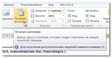
When you print a worksheet on multiple pages, the column or row headings are not visible on all of them. In our example, there are no month names on the second page. In such a situation, it is useful to duplicate the headings. To do this, follow these steps.

Select File > Page Setup.

Expand the Sheet tab.

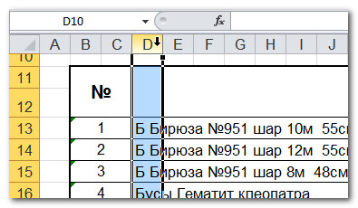
Click the button on the right side of the Rows To Repeat At Top field to collapse the dialog box and open access to the worksheet cells.

Click on the button for the first row of the sheet to select it.

Click the dialog box button again to expand it to its previous size (Fig. 12.12).

Rice. 12.12.Setting auto-repeat titles

The Columns To Repeat At Left field on the Sheet tab of the same dialog box allows you to specify the heading columns that should be repeated on the left side of each page. The checkboxes in the Print section of this tab add cell dividing lines, cell numbering, and enable black-and-white and draft printing modes. In the Page Order section, you can specify how pages are sorted when printing multi-page tables.

Click OK. Now the names of the months will be displayed on both pages.

Exercise 9: Setting a cell range

To print only part of a table, you don't have to filter it or hide rows and columns. You can simply specify the range of cells that should be printed. Notice that on the second sheet there is a large gap between the column headings and the table numbers. Let's eliminate it by excluding it from the print range empty lines 7-9.

1. Select lines 1 to 6.

   Click Ctrl key and drag the pointer over the buttons on lines 10-14 to add them to the existing selection, as shown in Fig. 12.13.

   Select the command File > Print Area > Set (File > Print Area > Set Print Area). Now only the selected lines will be printed. Check it out in preview mode.

Rice. 12.13.Setting the Print Range

Note

If, after completing step 3, you expand the Sheet tab of the Page Setup dialog box, you will see in the Print Area field a link 1:6;10:14, which corresponds to the lines highlighted in steps 1 and 2. That is, the print range You can also set using this field in the Page Settings dialog box. To reset the set print range, simply select the command File > Print Area > Clear Print Area.

The completed operations complete the settings for printing the Formula sheet. But in addition to the table, you need to print a chart that represents the data in graphical form. In the next exercise, you will configure the Chart worksheet settings and print it along with a table of source data.

Exercise 10: Customizing Charts

Sheets that are entirely occupied by diagrams have the same print options as standard ones. However, the Sheet tab of the Page Setup dialog box for these sheets has been replaced by the Chart tab.

Click on the spine of the Chart sheet.

Select File > Page Setup.

Expand the Diagram tab shown in Fig. 12.14.

Rice. 12.14.Chart Print Options

To make the diagram occupy the entire sheet, select the Scale To Fit Page switch.

Note

If the diagram will be printed on black and white printer, check the box next to Print in black and white.

Click OK.

All that remains is to output the sheets to the printer. To do this, follow these steps:

Press the Ctrl key and, without releasing it, click on the spine of the Formula sheet. The Chart sheet will remain active, but the Formula spine will turn white, indicating the selected status of the sheet. You can now print two sheets of paper at once using one print operation.

Select File > Print or click the Print button on the toolbar in Preview mode. A dialog box will open, shown in Fig. 12.15. It offers additional ways print range settings.

Note

To select several adjacent sheets, click on the spine of the first one, click Shift key and, without releasing it, click on the spine last sheet allocated group.

Rice. 12.15. Printing sheets

Make sure that in the Print Range section the All radio button is selected.

If you only want to print some pages, select the Page switch position (Page(s)) and enter the required numbers in the From and To counters.

Select the Active Sheets position of the Print What switch.

In Excel, unlike Word, very often tables with data do not correspond to A4 format. When preparing a document for printing, you should anticipate this moment and correctly set the boundaries of Excel sheets.

The developers of Excel foresaw the difficulties that arise when formatting a document for printing. They offer us 3 ways to solve this problem: 1. In the page settings, you can define and set your own parameters for placing the document on a certain number of sheets after printing. 2Page layout. Allows you to set the print area in Excel. Setting and fixing sheet boundaries for a document. 3Page mode. Allows you to freeze the print area in Excel. IN this mode You can control the borders of sheets and fix them on the document.

Setting Page Options

Open the Page Setup dialog box. Select the “Page Layout” tab and click on the corner in the “Page Settings” section

Here we can change the page orientation from portrait to landscape. You can also reduce or increase the print scale in Excel, which allows you to print a table on one sheet. Or print two pages on one Excel sheet. But here we sacrifice data sizes after printing. Therefore, it is better to set the data in the “place no more than on:” section. And specify in the parameters: “p. wide" and "p. in height" is the number of pages on which our document will fit after printing. You can set the quantity using the mouse or keyboard.

Basically, the width should be one page, and the height should be set to the maximum number. The program will not make any errors; it will automatically divide the tables into parts and optimize them for the actual remainder of the pages.

In the same dialog box, go to the “Fields” tab.

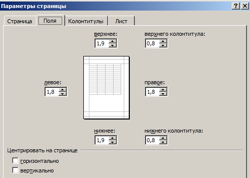
Here you can set the location of data and tables on the page. You also have the ability to control the size of the fields. You can also remove margins when printing an Excel table.

Please note the "Center" section below. Two useful options: horizontal or vertical. It's better to choose both options.

This small review pre-printing options large documents and in most cases there are enough tables. But it’s also worth familiarizing yourself with the page layout and page mode options. Their functions are very flexible and convenient for print preparation.

Page mode allows us to fix the boundaries of the document's printable area on all pages at the same time. It allows you to customize and optimize tables to fit the size and orientation of paper sheets.

In addition, this mode provides the most convenient preview before printing. After all, all pages from optimal scale, like medium-sized miniatures. The situation is completely under the user's control. Let's look at how to set how to increase, decrease or delete printable areas.

How to set print area in Excel?

To switch to the mode for managing borders and areas, you need to go to the “View” tab and in the book viewing mode section, select the “Page Mode” tool

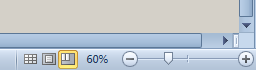
The second option is to click on the third switch in right side window status bars.

How to change print area in Excel?

To set the print area, you need to set and fix the boundaries of the page layout, which will separate all areas. To do this, in page mode, click on the blue dotted line while holding left key mouse, move the blue line to the desired position.

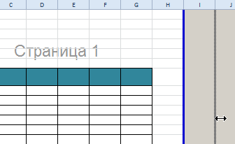
If the table extends beyond the white area, then everything that is in the gray area will not be printed. If in page mode all your data is in the gray area, then when printing from Excel it comes out empty page. You can force the print area to disappear by moving the boundaries between the gray and white fields.

In order to set the print area, you need to set and adjust the boundaries. How to add borders? Click on the cell that is located in the place where there should be a page break and select the “Insert page break” option.

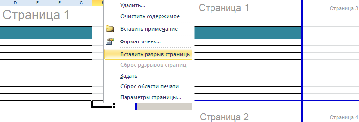
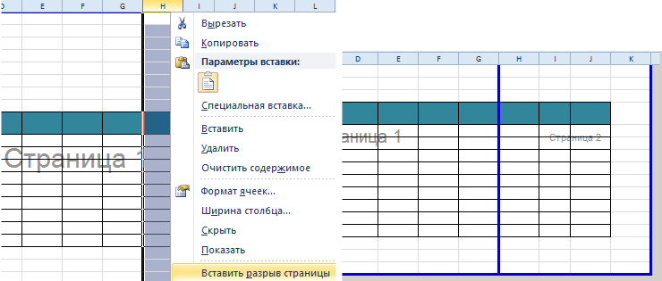
How to add only a vertical border? Right-click on the column where the border will be drawn and select the same option: “Insert page break.” When inserting a horizontal border, we proceed in the same way, only click on the row header.

Note. Note that there is a "Reset Page Breaks" option in the context menu. It allows you to remove all borders and make default settings. Use it to start over.

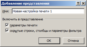
How do I save my print area settings?

All area settings can be saved in templates, so-called “Views”. This tool is located under page mode.

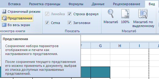
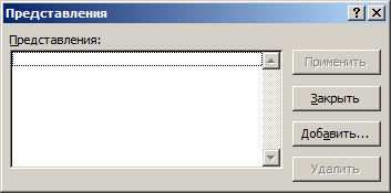
When you select the Views tool, the View Manager loads.

New versions of Excel since 2007 have effective means for preparing documents for printing. An Excel document is more specific in terms of organizing data for printing than Word document. Therefore, Excel tools for setting up and preparing documents for printing have big amount functions.

There are many printing options Excel workbooks. You can choose which part of the book to print, and how to arrange the information on the page.

In this lesson you will learn how to print sheets, books And selected cells. You'll also learn how to prepare books for printing, such as changing page orientation, scale, margins, printing headings, and page breaks.

Previous versions of Excel had a Workbook Preview feature that let you see what the workbook would look like when printed. You may notice that Excel 2010 does not have this feature. It hasn't actually disappeared, it's just that it's now connected to the Print window and forms a single panel that's in the File pop-up menu.

To see the Print panel:

1. Click on the File tab to open a pop-up menu.
2. Select Print. On the left will be the print settings settings, and on the right is the Document Preview panel.

1) Print button

When you're ready to print your book, click Print.

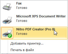
2) Printer

You may need to choose which printer to use if your computer is connected to multiple printing devices.

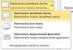
3) Print range(customization)

Here you can choose whether to print active sheets, the entire workbook, or a selection.

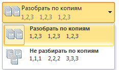
4) Disassemble/Do not disassemble into copies

If you are printing multiple copies, you can choose whether to collate the sheets or not.

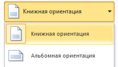
5) Orientation

Here you can select Book or Landscape orientation pages.

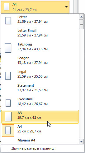
6) Paper size

Here you can select the paper size you want to use when printing.

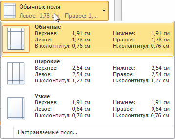
7) Fields

Here you can customize the fields. This is useful if part of the sheet is cut off by the printer.

8) Scale

Choose how to arrange your sheets on the printed page. You can print the actual size sheet, fit it onto one page, or fit all the rows or columns on one page.

9) Page

Click the arrow to see another page in the preview pane.

10) Preview

Allows you to see what the printed book will look like.

11) Show margins/Fit to page

The Fit to Page button is on the right. Click on it to zoom in and out of the image in the preview panel.

The Show Margins button is located to the left of the Fit to Page button. Click on it to configure the book margins.

To print active sheets:

If your book has multiple sheets, then you will have to decide whether to print the entire book or specific sheets. Excel gives you the option to print only active sheets. A sheet is considered active if it is selected.

To print the entire book:

To print a selection or set the print area:

Print Selection (sometimes called a print area) allows you to select specific cells to print.

You can also set the print area in advance on the Page Layout tab. This will cause a dotted line to appear around your selection. This way, you can see which cells will be printed while you work. To do this, simply select the cells you want to print and select Print Area on the Page Layout tab.

To change the page orientation:

Change the orientation to Portrait for the page to be vertical, or Landscape for the page to be horizontal. Portrait orientation useful when you need to fit more rows on a page, and Landscape when you need to fit more columns.

To fit a sheet onto one page:

To customize margins in the preview pane:

You may need to adjust the margins on the worksheet to help the information fit better on the page. You can do this in the preview panel.

1. Click on the File tab.
2. Select Print to open the print panel.
3. Click on the Show fields button. The fields will appear.
4. Hover your mouse over the field indicator; it will turn into a double arrow.
5. Clamp left button mouse and drag the field to the desired position.
6. Release the mouse button. The field has been changed.

To use page titles:

To insert a page break:

Greetings to all B&K employees! My question is this. Excel 2003 had convenient tool For visual settings fields before printing the table. Instead of specifying the size of the fields on the form in numerical form, you could enter preview mode, show the boundaries of the printable area and move them manually using the mouse. This was the most visual way to layout pages. Unfortunately, I did not find such a tool in Excel 2010, nor did I find the preview command itself. Have the developers really removed such a wonderful opportunity? Tell me how I can replace the margin setting tool in Excel 2010. Thank you.

Nikolay Betsenny, accountant, Kharkov

AnswersNikolay KARPENKO, Ph.D. tech. Sciences, Associate Professor of the Department of Applied Mathematics and information technologies Kharkov National Academy of Municipal Economy

IN new program Excel 2010 print and preview tool is one. But all the features characteristic of previous versions of this program remain, including the means of visually adjusting the width of the fields. They are just located in a different place. Therefore, I propose to go through the basic printing parameters of Excel 2010, and along the way, find out how to use the margin width adjustment tools. For this we need any document. For example, a regular invoice form, which I created based on a sheet of format " A5 " And now our task is to configure the printing settings for this document. Let's do this.

1. Open the document, click on the button “ File » main menu of the program Excel 2010.

2. Select the item “ Seal " The settings window shown in Fig. will open. 1.

In the center of the window, next to the list of menu items, there is an area for defining printing parameters. On the right in the window is shown general form table, how it will look on the page. In essence, this is an analogue of the program preview mode Excel 2003. Please note that by default the document is shown without visual margin markings. To enable it we do this.

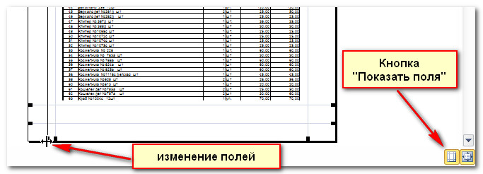
1. In the lower right corner of the print settings window we find two buttons. One of them (on the left) is called “ Show fields ", another - " Fit to page».

2. Click on the button “ Show fields ", lines will appear around the perimeter of the page to adjust the margins (Fig. 1). Now, to change the width of the margins, you need to use the mouse to move the lines so that the document fits completely on the page. Convenient and clear.

And, since we are talking about printing, I propose to see what other opportunities it offers in this regard. Excel 2010. To do this, let's return to the window in Fig. 1. Most of the parameters of this window were in previous version programs. Although there were useful news. But first things first.

Group "Print" "consists of two controls. Click on the button Seal » starts printing the document to the current (active) printer. In the window " Copies » You can specify the number of copies of the printout.

Click on the list " Printer » opens all available printers on this computer. The printer itself does not need to be physically present. The main thing is that the so-called drivers for this device are installed. Then the document will be formatted taking into account the characteristics of a particular printer.

Advice When working with a document, make active the printer where the printout will be made. Otherwise appearance document on screen may differ from what appears on paper.

The group of greatest interest to an accountant is “ Settings " It has six elements.

The first parameter of the group specifies the workbook objects that need to be printed.Excel 2010 offers three options: "Print active sheets», « Print the entire book" And " Print selection"(Fig. 2). With this, I think everything is clear. But on the checkbox “Ignore print area“I advise you to pay attention. In practice, accounting spreadsheets are often accompanied by intermediate calculations. The results of these calculations often do not need to be printed. To selectively print worksheet data, it is convenient to use the so-called current document print area. IN Excel 2010 print area can be set in the menu "Page layout"(icon "Print area" group " Page Options"). If at some point you need to print the document along with intermediate calculations, you will not have to cancel the print area. Just turn on the "Ignore print area» and print the document. In previous versionsExcel such features were available through the menu "File → Print Area → Set», « File → Print Area → Remove».

Next in the “Settings” group " followed by the parameter " Pages: " It can indicate the number of the first and last page that need to be sent for printing.

Parameter " Disassemble into copies» convenient to use so as not to reposition the paper after printing. You can order printing from the first page to the last or vice versa. The specific choice depends on the characteristics of the printing device.

The page orientation list consists of two parameters: "Portrait orientation" And " Landscape orientation" In addition, these parameters can be set in the printer settings. There is no difference.

The fourth parameter from the top of the group “ Settings » allows you to select the size of the printed sheet. It could be " A4", "A5 ", custom size, etc. The number of options offered depends on the printer model. In this sense Excel settings 2003 and Excel 2010 are no different.

And here is the parameter “ Custom fields» appeared only in new version programs. Clicking this option opens a menu of six items (Figure 3). The first three of them are fixed values for page margin sizes (" Regular", "Wide" or "Narrow" "). The option “", and it's very convenient. The point is that the field sizes Excel stores individually for each workbook sheet. Therefore, in Excel 2003, margin parameters had to be set for each sheet separately. Now everything is easier. If in workbook some identical documents(for example, reports for each month of the current year), you can configure fields for only one sheet. And for the rest, select the option “Last user value».

Click on the hyperlink "Custom fields..."opens a window"Page settings"immediately on the tab" Fields " In this window you can also set field values, but in numerical form.

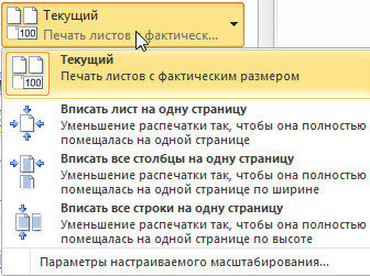
The last parameter of the group " Settings » is designed to automatically scale a document when printing it. Here is the programExcel 2010 offers several useful features(Fig. 4):

- "Current" ", prints the document without changing the scale;

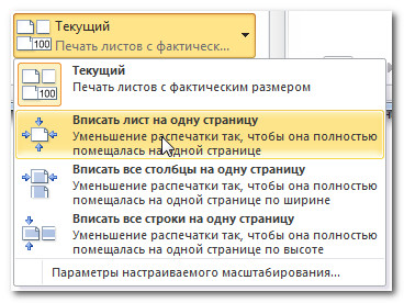
— « Fit the sheet to one page", will automatically select the scale of the document so that it fits on one page;

— « Fit all columns on one page", selects the document scale so that it fits the width of the page;

— « Fit all lines on one page", scales the document to fit the height of the page. Auto-scaling of documents by page height and width - new features Excel 2010;

— « Custom scaling options...", opens the window "Page settings", where you can configure print settings manually.

As you can see, in terms of printing settings Excel 2010 inherited all the features from the previous version of this program, including the means of visually adjusting fields. At the same time, new automatic scaling modes and improved field settings tools will help the accountant quickly cope with the task of preparing reports for printing.