Example of an Excel table with formulas. Basic Excel functions to work with

Microsoft Excel the most popular office program to work with data in tabular form, and therefore almost every user, even a beginner, simply must be able to work in this program. Working in Excel means not only viewing data, but also operating with this data, and for this they come to your aid functions, which we will talk about today.

I would like to immediately note that we will consider all examples in Microsoft Office 2010.

Today we will look at some of the most common Excel functions that you use very often. They are actually very simple, but for some reason some people are not even aware of their existence.

Note! Today’s material is devoted to the built-in functions that are present in Excel by default; today we will not consider macros or VBA programs; we have already touched on the topic once on this site VBA Excel in the article - Denying access to an Excel sheet using a password, if you are interested, you can take a look.

Let's get started.

Excel Function - Concatenate

This function connects several columns into one, for example, your last name, first name, middle name are located in a separate column, but you would like to combine them into one. You can also use this function for other purposes, but I hope its meaning is clear, an example is below. In order to call this function, you need to write = concatenate(column1; column2, etc.) in a separate cell, or click the button on the panel “ insert function» and type concatenate in the search, and only then select the fields in the graphical interface.

Excel function - VLOOKUP

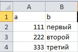
This function stands for " Vertical view"and it is useful because it can be used to search for data in other sheets or Excel documents according to a certain key field. For example, you have two tables containing one identical field, but the remaining columns are different and you would like to copy data from one table to another for this key field:

Table 1

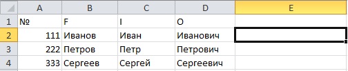
table 2

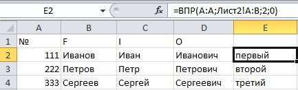
You proceed as in the previous example, or write or select through the GUI, for example:

There should be no problems with describing the fields, everything is written there. Next, click “OK” and get the result:

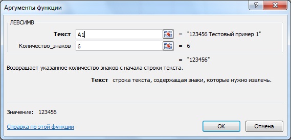
Excel Functions – RightSim and LeftSim

These functions simply cut out the specified number of characters on the right or left (I think the name makes it clear). For example, it is required when you need, for example, to get an index from an address into a separate field, and the index is meant to go at the beginning of the line, or any other number or personal account who has what needs, for example:

Excel Function - If

This is a regular function for checking an expression or value. Sometimes it's useful. For example, we need a column C record the value "More than" or "Less than" based on field comparison A And B those. for example, if A is greater than B, then we write “More”; if less, then we write “Less” accordingly:

I think that’s enough for today, and I think the principle is clear, i.e. in the function selection window, all functions are grouped by purpose (category) and with detailed description You already know how the function window is called up, but I’ll remind you anyway, on the panel click “Insert function” and look for the function you need and that’s it.

I hope all of the examples listed above will be useful to you.

Alexey Vasiliev “Excel 2010 with examples” BHV-Petersburg, 2010, 432 pages (31.6 mb. pdf)

The book provides specific examples, educational and practical, by looking at which you will learn one of the most popular office applications – Microsoft Office 2010. All examples are based on Excel versions 2010. Talks about user graphical interface, technical techniques, settings, hyperlinks, printing tools, formatting and application of styles, data processing methods, programming in the VBA environment and many other questions that arise for the user.

Examples of solutions are given applied problems from different sections of natural science: mathematical, physical, statistical, economics, as well as logistics problems. The book consists of six parts, each of which belongs to a specific group of Excel 2010 functionality. In turn, each part consists of five chapters, examples in which are grouped according to the issues addressed in each chapter. More details on the questions and examples presented in the book “Excel 2010 by Example” can be found in the table of contents.
ISBN 978-5-9775-0578-9

PART I. INTERFACE 3

Chapter 1. Working window 5
Example 1.1. Changing the data display scale 5
Example 1.2. Paged view 10
Example 1.3. Panel quick access 13
Example 1.4. Name field 18
Example 1.5. Formula bar 20
Example 1.6. Status bar 23
Example 1.7. Full screen mode 25
Example 1.8. Displaying grid and indexing fields 27
Example 1.9. Using the Settings Window 29
Example 1.10. Color scheme 31

Chapter 2. Tape 33
Example 2.1. Ribbon Tabs 33
Example 2.2. Show or hide the ribbon 39
Example 2.3. Add Ribbon Groups to the Quick Access Toolbar 40
Example 2.4. Active Tape Group Label 41
Example 2.5. Ribbon customization 45
Example 2.6. Contextual Ribbon Tabs 50

Chapter 3. Areas 53
Example 3.1. Selecting areas 53
Example 3.2. Working with the selected area 56
Example 3.3. Collapse and expand rows and columns 57
Example 3.4. Resizing Cells 62
Example 3.5. Dividing the work area into parts 65

Chapter 4. Sheets 76
Example 4.1. Adding and removing sheets 76
Example 4.2. Default number of sheets 78
Example 4.3. Renaming and highlighting sheets 80
Example 4.4. Hiding and showing sheets 81
Example 4.5. Displaying sheet spines 84
Example 4.6. Adding a background 86

Chapter 5. Books 88
Example 5.1. Creating a new working document 88
Example 5.2. Saving a document 91
Example 5.3. Creating a Template 95
Example 5.4. Working directory 115
Example 5.5. Automatic download file 116
Example 5.6. Connecting add-ons 117
Example 5.7. Window management 119
Example 5.8. Working space 124

PART II. RESOURCES 127

Chapter 6. Settings 129
Example 6.1. Switching to row-column mode 129
Example 6.2. Relative links in row-column format 131
Example 6.3. Mixed links in row-column format 133
Example 6.4. References to cell ranges in row-column format 134
Example 6.5. Default font 135
Example 6.6. Calculating values ​​136
Example 6.7. Error display 137
Example 6.8. Displaying formulas in cells 138
Example 6.9. Data entry and editing mode 139
Example 6.10. Data display and calculation accuracy 140

Chapter 7. Hyperlinks 141
Example 7.1. Inserting hyperlinks into a document 141
Example 7.2. Adding a Comment to a Hyperlink 143
Example 7.3. Hyperlink to cell range 145
Example 7.4. Link via name 147
Example 7.5. Hyperlink to external document 148
Example 7.6. Hyperlink to new document 151
Example 7.7. Hyperlink to Internet page 151
Example 7.8. Hyperlink to send mail 153
Example 7.9. Image based hyperlink 154
Example 7.10. Using Functions to Create Hyperlinks 156

Chapter 8. Notes and Boxes 159
Example 8.1. Creating a note 159
Example 8.2. Mode permanent display notes 161
Example 8.3. Application settings for displaying notes 163
Example 8.4. Setting the note type 164
Example 8.5. Graphic forms 168
Example 8.6. Structural diagrams 172
Example 8.7. Text fields 175
Example 8.8. Literary text 176
Example 8.9. Sparklines 179

Chapter 9. Seal 182
Example 9.1. Printing a document 182
Example 9.2. Creating Headers and Footers 187
Example 9.3. Icons of the Working with Headers and Footers tab 190
Example 9.4. Adding special fields to headers and footers 192
Example 9.5. Pagination 193
Example 9.6. Basic Print Settings 197

Chapter 10. Add-ins 199
Example 10.1. Solving trigonometric equation 199
Example 10.2. Solution search utility settings 203
Example 10.3. Generation random numbers 205
Example 10.4. Totalizer 207
Example 10.5. Substitution Wizard 210

PART III. FORMATS 213

Chapter 11. Number Formats 215
Example 11.1. Formatting Numeric Data 215
Example 11.2. Using exponential format 218
Example 11.3. Using the Fractional Format 219
Example 11.4. Using monetary and financial formats 221
Example 11.5. Percentage format 222
Example 11.6. Time and date format 222

Chapter 12. User Formats 225
Example 12.1. Simple number format 225
Example 12.2. Scientific User Format 228
Example 12.3. User Fractional Format 229
Example 12.4. Inserting symbols and text 230
Example 12.5. Special formats 231
Example 12.6. Template for the meanings of different signs 232
Example 12.7. Template with highlighting 234
Example 12.8. Conditional format based on pattern 235

Chapter 13. Conditional Formats 236
Example 13.1. Conditional formatting based on value comparison 236
Example 13.2. Checking for belonging to the range of values ​​240
Example 13.3. Formula 242 format
Example 13.4. Using pictograms in 248 format
Example 13.5. Format using color and graphic indicators 251
Example 13.6. Formats based statistical parameters 253

Chapter 14: General Formatting 257
Example 14.1. Aligning data in cell 257
Example 14.2. Font settings 258
Example 14.3. Cell Borders 258
Example 14.4. Using Fill and Pattern 260
Example 14.5. Protection mode 261
Example 14.6. Copying formats 263
Example 14.7. Creating groups 265

Chapter 15: Styles and Automatic Formatting 268
Example 15.1. Applying built-in table styles 268
Example 15.2. Working with styled tables 272
Example 15.3. Creating a New Table Style 277
Example 15.4. Using built-in cell styles 279
Example 15.5. Creating a new style 283

PART IV. DATA 285

Chapter 16. Entering and editing data 287
Example 16.1. Fill a range of cells the same values 287
Example 16.2. Automatic filling cells 290
Example 16.3. Entering formulas 293
Example 16.4. Copying formulas 295
Example 16.5. Array formulas 299
Example 16.6. Cell references in different sheets 299
Example 16.7. Links to cells in different books 300
Example 16.8. Circular links 301
Example 16.9. Using Numeric Formulas 302

Chapter 17. Built-in Excel functions 304
Example 17.1. Inserting inline function 304
Example 17.2. Trigonometric and hyperbolic functions 308
Example 17.3. Calculating series 311
Example 17.4. Working with matrices 314
Example 17.5. Calculating sums 316
Example 17.6. Logic functions 320
Example 17.7. Statistical Functions 321
Example 17.8. Functions for working with text, date and time 325

Chapter 18. Diagrams 328
Example 18.1. Quick creation diagrams 328
Example 18.2. Changing the chart type 334
Example 18.3. Editing a Chart Area 337
Example 18.4. Settings for individual chart elements 345
Example 18.5. Show empty and hidden cells 350
Example 18.6. Creating a Chart Template 353
Example 18.7. Using specific settings for different data series 354
Example 18.8. Trend line 356

Chapter 19 Scenario Analysis 359
Example 19.1. Lookup tables 359
Example 19.2. Scenario Manager 366
Example 19.3. Creating a Pivot Table 373
Example 19.4. Editing a PivotTable 377
Example 19.5. Creating a PivotChart 379
Example 19.6. Parameter selection utility 382

Chapter 20. Correcting Errors 384
Example 20.1. Basic errors 384
Example 20.2. Control elements of the Formula dependencies group 385
Example 20.3. Bug Tracking 386
Example 20.4. Error Control Utility 386
Example 20.5. Checking the control value 389

PART V. PROGRAMS (see CD-ROM, page 1) 393

Chapter 21. VBA language 2
Example 21.1. Selecting cells and ranges 2
Example 21.2. Changing cell values ​​7
Example 21.3. Cell and Range Formatting Options 11
Example 21.4. Enter using software methods formulas in cells 15
Example 21.5. Using Excel 18 Built-in Functions
Example 21.6. Conditional statements and loop statements 19

Chapter 22. VBA Editor 25
Example 22.1. Displaying auxiliary windows and toolbars 25
Example 22.2. Inserting modules and forms 30
Example 22.3. Project Window 32
Example 22.4. Properties window 33
Example 22.5. Editor settings 35
Example 22.6. Compiling and debugging projects 37
Example 22.7. Running Macros 38
Example 22.8. Connecting links 39

Chapter 23. User Functions 41
Example 23.1. Creating a Function in the VBA Editor 41
Example 23.2. Factorial calculation 45
Example 23.3. Sine calculation 47
Example 23.4. Creating a Piecewise Smooth Function 50
Example 23.5. Calculating Fibonacci number 51

Chapter 24. Forms 54
Example 24.1. Creating a Simple Form 54
Example 24.2. Using 64 fields
Example 24.3. Form with option 69
Example 24.4. Form with switch 71
Example 24.5. Tabbed form 73

Chapter 25. Macros 76
Example 25.1. Macro recording 76
Example 25.2. Optimization program code 81
Example 25.3. Record a macro with relative links 82
Example 25.4. Adding a Macro Run Button
to the quick access panel 87
Example 25.5. Security Settings 89

PART VI. TASKS (see CD-ROM, page 91) 395

Chapter 26. Equations and systems 92
Example 26.1. Solving an equation using the Parameter Selection utility 92
Example 26.2. Solving the equation in automatic mode 94
Example 26.3. Half division method 96
Example 26.4. Successive Approximation Method 101
Example 26.5. Solving a system of equations 107
Example 26.6. Search for a solution on the interval 109
Example 26.7. System linear equations 110

Chapter 27. Probability theory and statistics 112
Example 27.1. Numerical characteristics of a discrete random variable 112
Example 27.2. Correlation of random variables 114
Example 27.3. Sports lotto game 117
Example 27.4. Distribution function 119
Example 27.5. Probability of realization of a discrete random variable 122
Example 27.6. Correlation statistics 124
Example 27.7. Descriptive statistics 126

Chapter 28. Economics and finance 128
Example 28.1. Production function 128
Example 28.2. Cost of investment projects 132
Example 28.3. Internal rate of return 135
Example 28.4. Future value of investment 140
Example 28.5. Loan payments 142
Example 28.6. Depreciation calculation 146
Example 28.7. Security Analysis 151
Example 28.8. Volatile financial flows 159

Chapter 29. Logistics and optimization problems 162
Example 29.1. Extremum objective function with restrictions in the form of equalities 162
Example 29.2. Determination of the number of two brigades 165
Example 29.3. Conditional extremum nonlinear function 170
Example 29.4. Extremum is implicit given function 172
Example 29.5. Conditional extremum of an implicitly specified function 174

Chapter 30. Physics 177
Example 30.1. Body on an inclined plane 177
Example 30.2. Calculation of friction coefficient 181
Example 30.3. Electron in an external field 184
Example 30.4. Magnification of the converging lens 189
Example 30.5. Longitudinal lens magnification 190
Example 30.6. Ideal gas pressure 191
Example 30.7. Body volume under the piston 192
Example 30.8. Calculation of resistor resistance 195
Example 30.9. Calculation internal resistance 199
Example 30.10. Determination of air humidity 201

Excel 2010 with examples. Video

It is important for an SEO specialist to be able to work with data, sort it, filter it, and transform it. For many functions, standard Excel is convenient. In this article we will look at the most basic functions of Excel, which every specialist should master to work productively.

Source file (download CSV file, 1.5 KB)

As initial data, consider a file of the “Distribution” type, which contains promoted search queries with the indication (Fig. 1):

• Promoted URL
• Relevant URL
• Positions in Yandex
• Frequencies
• Google Positions
• Missing words in Title tag
• Others

Rice. 1. Initial table for work.

Sort by any field

For this operation it will be enough to transform work area table with headings (Fig. 2). After that, sorting by any of the fields (Fig. 3) will be available by clicking on the square with the arrow to the right of the column name.

Rice. 2. Insert a table with headers in Excel file for further work.

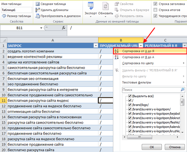
Rice. 3. Sort text fields from “A to Z” and from “Z to A” in a table in Excel. For numeric fields, sorting from minimum to maximum value and vice versa is available.

Highlighting duplicates or unique values

Often, search queries in a table may duplicate each other, or vice versa, you need to find all unique queries in order to compare two lists. For this, the “Conditional Formatting” function (Fig. 4) and creating a new rule for it will be useful. Before clicking on the “Conditional Formatting” button, you need to select the area that will be affected by further work for highlighting/formatting values. In our case, the entire first column is selected.

Rice. 4. Create a new rule for conditionally formatting the selected area.

Afterwards, select “Format only unique or repeating values”, set the type, in the example it is “Repeating” and Format, in the example it is orange (Fig. 5).

Rice. 5. Set the color orange to format duplicate values ​​in the selection.

Removing Duplicate Values

After applying the rule, repeating values ​​in the selected area will be highlighted in orange (Fig. 6). By this color you can sort in the table and work on or delete these lines.

Rice. 6. Removing Duplicate key query after sorting by orange color in the table.

Highlighting the colors of values ​​in a range

For color highlighting values ​​in a given range, it is also convenient to use conditional formatting. To do this, we need to select the columns or cells we are interested in and create a new rule for the “Conditional Formatting” function, then select “Format only cells that contain” and set the cell values ​​in the required range, for example, from 1 to 10 (Fig. 7) .

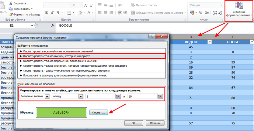
Rice. 7. Set green formatting for cells between 1 and 10 using the conditional formatting function.

Rice. 8. An example of highlighting the required cells in the table with positions in the TOP-10 in green.

Search for queries with a given word

Often, you need to quickly find and select all queries that contain a given word, say, the word “site”. To do this, you can similarly use the conditional formatting function to set the format for cells that contain the text “site” (Fig. 9).

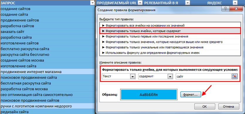
Rice. 9. Example quick search and work with search queries, which contain the word “site”.

Calculating the value using the formula

The table also makes it convenient to calculate any indicator using a formula, based on the values ​​in other indicators. In particular, you can calculate the predicted budget as the average value between the budget from the SeoPult and MegaIndex systems (Fig. 10). To do this, just set the formula for the first cell of the table and clear the value for the entire table.

Rice. 10. Calculation of the link budget, in Excel spreadsheet based on values ​​from aggregators SeoPult and MegaIndex.

Copying values ​​from a column calculated using a formula

If you now go to copy the values ​​from the calculated column “To references” to another sheet or to another file, you will encounter minor difficulties. Since the values ​​are calculated using a formula that is “stuck” in the cell, simply copying CTRL+C and CTRL+V will be incorrect (it is the formula that is copied, not the numbers) and you will need to use the “Paste Special” function. Step by step it looks like this (Fig. 11):

1. Select the values ​​that you need to copy with the mouse.
2. Press CTRL+C.
3. Next, select the cell from which you plan to insert.
4. Click the edit mouse button.
5. Select "Paste Special".
6. Set "Insert values".

Rice. 11. Function special insert in Excel for copying and pasting exactly numerical values, and not the original formula by which they were calculated.

IN in this case, exactly the values ​​from the cell will be copied, and not the formula by which they were calculated.

Comparing values ​​in two columns

To understand whether the page being promoted and the page that is relevant in the search results coincide (and a number of other tasks), you need to use logical function"IF". You need to add a comparison column “Does it match?” into the table and insert a function into the first cell of this column, the following sequence actions: “Formulas”, then “Logical”, then “IF” (Fig. 12). Set logical expression, let's say [@[ PROMOTED URL]]=[@[ RELEVANT IN ME]]" and the function values ​​are "1" and "0". To speed up the process, you can immediately insert a function into the column:

IF([@[ PROMOTED URL]]=[@[ RELEVANT IN I]];1;0)

Rice. 12. Call the logical "IF" function in Excel to compare values ​​in two columns.

After clicking the “OK” button, the column will be filled with the values ​​“0” (if the pages do not match) and “1” if the values ​​do match. This will allow you to quickly find all queries for which the relevant and promoted document do not match, and begin analysis possible reasons this behavior.

Using formulas: average and sum of values ​​in cells

To calculate the average value of a parameter (say, the average position in Yandex for all queries or mid frequency requests), as well as the sum of values ​​(say, total exact frequency or total link budget), you need to use mathematical functions. The most popular are: calculating the average, calculating the median, calculating the sum of values ​​in a column.

In Fig. Figure 13 shows the sequence of actions for inserting a function. First, you need to select the cell in which you want to display the final calculated value, then select the function you are interested in and the range of values ​​over which you plan to perform calculations.

Rice. 13. Select a cell and insert the desired one mathematical function cell.

After searching required function, you need to set the arguments (the values ​​with which the function will work) and click “OK”. If you did everything correctly, the value will be calculated and inserted automatically. Examples of inserting the functions of the average value (Fig. 14) and the sum of values ​​(Fig. 15) are presented in the illustrations below.

Rice. 14. Inserting a function for calculating the average value of cells for the “YANDEX” column.

Rice. 15. Inserting the “AutoSum” mathematical function to quickly calculate the sum of values ​​in a column.

Excel has a lot of tools in its arsenal various functions, which may be useful to an SEO specialist, you can search for them by entering the first letters of the required operation into the function search bar. Some useful functions may also include the following:

• Finding the maximum and minimum value in a collumn.
• Using logical operators: “AND”, “OR”, “IF”, “NOT”.
• Working with date and time, output current date according to the calendar.
• Sum, sum of values ​​with condition, median.

Setting the cell format

To set the required cell format (numeric, monetary, financial, time, percentage, text, etc.), just use the “Format Cells” function, first selecting the formatting area of ​​interest and clicking right button mouse (Fig. 16), in the pop-up modal window Click “Format Cells...”.

Rice. 16. An example of calling the “Shape Cells” function for a selected area.

After specifying required format values ​​in the cells, click “OK” (Fig. 17) and the selected format will be applied in the selected area. Using this function, you can get rid of the forced conversion of some values ​​into date format in Excel and set the most visual and appropriate format for the data (for example, display instead of 0.1 → 10%, add digit groups of digits large values 340339493 → 340 339 493, hide extra decimal places 5.100015 → 5.1).

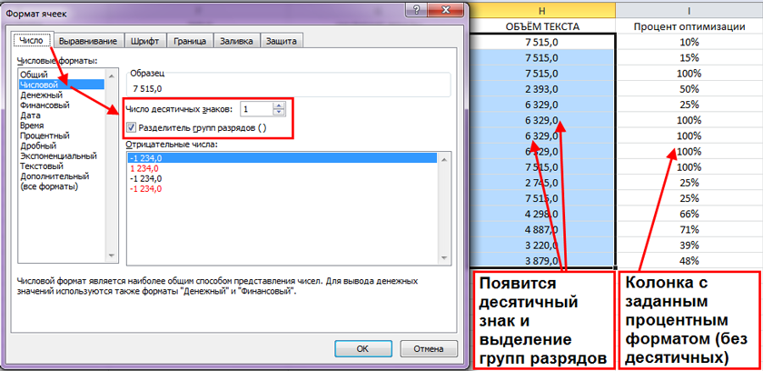
Rice. 17. Task of two various formats(numeric and percentage) for two adjacent columns.

Fixing the position of one of the cells in a formula

If you need to fix the position (cell) for one of the variables in the formula, then you simply need to replace the value of the form =F2 in the formula itself with the value =$F$2 (insert a dollar sign). After which, you will be able to “stretch” formulas for the entire row or column, fixing one of the variables (cells). Usage example:

Value=$C$36+F13*2.2

* It's worth noting that the conditional formatting feature is only fast on small to medium-sized tables and doesn't handle large data sets well.

Creating a calendar in Excel for the whole year indicating holidays and weekends. You can immediately download a calendar in Excel, or spend 15 minutes and learn how to make it yourself, while simultaneously discovering new Excel features.

Sometimes you have to process a large set of statistical data. Often in these cases it is necessary to discard unreliable values, experimental errors - outlier points. And it’s good when the sample size is 10-20 values. How to process data on 100, 1000 or more large samples? This add-on will help you!

Many Excel users We also do not recommend using merged cells, as this can lead to the problems described in this article. However, you should not be so categorical; the main thing is to know how to avoid them and be able to use alternatives.

Since the advent of named styles in Excel (since version 2007), few people have paid due attention to this tool. But in vain, since named styles save time on document formatting and give it a unified “corporate” style

When working with data in Excel, you may need to organize it. For example, in a large organization you need a list of employees in alphabetical order names, as well as lists of them in descending or ascending order of length of service, age or salary. To solve this problem, you do not need to enter data multiple times. Using Excel's sorting mechanism, it's easy to sort your existing data into the order you want.

Excel sheets, consisting of cells, are themselves tables, in which the leftmost column already contains row numbers, and in top line– letters indicating the names of the columns. But in practice, tables of a certain size are required, that is, containing given number rows and columns.

The Quick Access Toolbar is necessary for those who often switch tabs on the ribbon because the required command is not on the screen. When you switch to any tab, this panel always remains on the screen, and if you place frequently used commands on it, they will always be at hand, which will significantly increase the speed of your work.

This article describes basic actions with worksheet elements, such as: moving through worksheet cells, selecting worksheet elements, selecting ranges of cells, selecting rows, columns, selecting all worksheet cells, copying and moving, inserting rows or columns, deleting rows or columns , changing the column width and row height.

Pivot tables are one of the the most powerful tools for data analysis. Using it, you can quickly consolidate large amounts of data and instantly analyze information from different sides. Possibilities pivot tables allow you to group data in design mode, make subtotals for different fields, and much more.