Which logical expression is simple? Work in groups on the computer. Role-playing game. Problem “calculating the cost of telephone conversations”

1. Conditional formatting

The simplest logic. If the contents of the cell are greater (less than, equal, not equal, etc.) certain value, then - a certain formatting is triggered for this cell (filling with the desired color, font color and style, borders, etc.)

Select the cells that should automatically change their color and select from the menuFormat - Conditional Formatting(Format - Conditional formatting).

In the window that opens, you can set conditions and then click the button Format , cell formatting options if the condition is met:

2. Conditional formatting with formulas

You can make the criteria for checking conditional formatting more complex if you check not the value, but the formula. In this case, you can check some cells and format others. This is how, for example, you can highlight all cells with values greater than the average:

3. IF function

IF - Very interesting feature, which allows you to display one value in a cell if a user-specified condition is met and another value if the condition is not met. The function has three arguments:

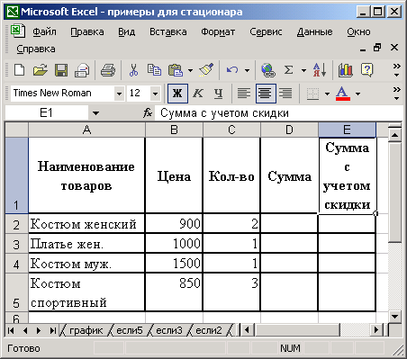
Let's look at a real-life example. We have the following table:

The solution is to use the function for calculation IF with the following parameters:

That is, if the quantity exceeds 5, then the person does not pay the full price (B2*C2), but only 90% of it (B2*C2*0.9).

4. Nested IFs

By itself, one IF function can only test one condition. Therefore, in the case when it is necessary to check several conditions at once, you have to nest one IF function within another. It looks something like this:

IN in this example The speed of the vehicle is checked. If it is more than 110, then the warning “Too fast!” is displayed. Otherwise, it checks to see if the driver is driving too slowly, and if not, the message “Everything is correct!” is displayed.

Excel allows you to nest IF functions within each other up to 7 times inclusive. Although the sight of such a formula will most likely cause a slight hiccup.

5. IF + AND + OR (IF,AND,OR)

AND and OR functions from the Logic category can significantly improve the visibility and understandability of complex logical checks. The previous example with speed checking could be implemented much more compactly and beautifully, for example, like this:

6. COUNTIF and SUMMIF functions(COUNTIF, SUMIF)

These functions should not be looked for in the category Logical, and in the categories Statistical and Mathematical , respectively (or in a complete alphabetical list).

COUNTIF - counts the number of cells in the range that satisfy a given condition, and SUMIF - sums their values:

Boolean expressions

Boolean expressions in Excel are used to write conditions that compare numbers, functions, formulas, text, or Boolean values. Any logical expression must contain at least one comparison operator, which defines the relationship between the elements of the logical expression.

Below is a list of Excel comparison operators:

The result of a logical expression is the logical value TRUE (1) or the logical value FALSE (0).

IF function

Function IF is a function that allows you to display one value in a cell if a user-specified condition is met and another value if the condition is not met.

Syntax:

IF(log_expression; value_if_true; value_if_false)

Move cursor to cell D2 . Use the function wizard to select from a category brain teaser IF function

(Fig. 27), and then click on the OK button. Dialog window Function Arguments . (Fig. 28) contains three input fields In field_ Log expression it is necessary to enter a condition that determines whether the quantity of goods sold exceeds 5 pcs., therefore, enter in this field C2>5 . In field Value_if_true. you need to enter a formula that calculates the cost of the product taking into account the discount, then enter in this field B2*C2-B2*C2*0.1 In field it is necessary to enter a condition that determines whether the quantity of goods sold exceeds 5 pcs., therefore, enter in this field Value_if_false it is necessary to enter a formula that calculates the cost of the product without taking into account the discount (condition-False), then enter in this field B2*C2

(see Fig. 29). Now let's click on the button .

OK. IF Copy the resulting formula into adjacent cells. The results of formula calculations are shown in Fig. thirty Functions can be nested inside each other as value_if_true and value_if_false arguments. Using nested functions like this.

More complex checks can be constructed. Let's look at examples of how to use a nested function

Determine the amount for which goods of each type were sold, taking into account the discount (amount including discount = amount - amount * discount). The discount is calculated according to the following principle: if goods are sold for an amount of more than 2500 UAH, then the discount will be 5%, if goods are sold for an amount less than 1100 UAH, then the discount will be 0%, in other cases the discount will be 2%.

In order to complete the first point of the task, you must enter the cell D2 enter the formula =C2*B2.

In order to calculate the discount amount we will use a nested function IF, since there are three options for calculating the discount.

Move the cursor to the cell E2 and using the function wizard, enter the following formula (Fig. 33 – 34). The solution results are shown in Fig. 35.

Click here

Rice. 35

OR, AND functions

OK. AND and function OR from category Use the function wizard to select from a category can significantly improve the visibility and understandability of complex logical checks. Function OR and function AND allow you to specify several conditions in the formula at the same time, i.e. make it possible to create complex logical expressions. These features work in combination with simple operators comparisons. Functions AND And OR can have up to 30 boolean arguments and have the syntax:

OR(boolean_value1, boolean_value2, ...)

AND(boolean_value1; boolean_value2; ...)

Function Arguments AND, OR can be boolean expressions, arrays, or cell references containing boolean values.

Function OR TRUE, if at least one of the logical expressions is true, and the function AND returns a boolean value TRUE, only if all Boolean expressions are true.

Suppose you want to display the message "Traffic Light" if the contents of cell B4 are either "red", "green", or "yellow".

If it contains any other information, then the message “This is not a traffic light!!!” must be displayed.IF(OR(B4="green";B4="green""red""yellow"

);"Traffic light"; "This is not a traffic light!!!" Suppose you want to display the contents of a cell B4<=B4<=100), и сообщение "Значение вне интервала" в противном случае.

, if it contains a number strictly between 1 and 100 (1<=100); B4; «Значение вне интервала»)

IF(AND(B4>=1; B4

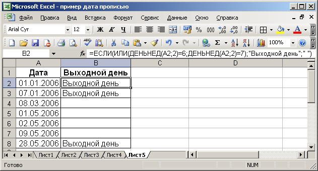
There is a list of dates, you need to determine whether the entered date is a holiday. Solutions to the problem in Fig. 36 Formula in cell AT 2

can be entered from the keyboard (you must remember the syntax of the nested functions used) or using the function wizard. Let's look at how to enter a formula using the Function Wizard: Move the cursor to the cell AT 2, The results of formula calculations are shown in Fig. thirty.

Click on the insert function button and select the function in the logical category In field_ Log Let's click in the field functions If, and then click on the down arrow in the formula bar and select Other features Use the function wizard to select from a category you can select a function OR.

Click on the insert function button and select the function in the logical category Boolean_expression_1 functions OR, and then click on the down arrow in the formula bar and select Other functions. In category Date and time select a function WEEKDAY and in the field Date_in_number_format let's introduce A2, and in the field Type let's introduce 2 .

OR OR, in order to finish entering the condition in the first field of this function (type = 6).

Click on the insert function button and select the function in the logical category Logical_expression_2 functions OR and repeat steps 3 and 4 to introduce the second condition WEEKDAY(A2,2)=7 .

In the formula bar, click inside the word IF and thus we can return to the function dialog box IF, in order to finish entering the formula (in the field . enter Day off, in field B2*C2-B2*C2*0.1 enter a space).

Information about the results of the first module control and student attendance at classes is displayed in the table, see Fig. 38. The following information must be displayed: If the student’s grade point average is less than or equal to 3.5 and he missed more than 49 hours of classes for an unexcused reason, then it is necessary to call the parents to the dean’s office; If the student’s GPA is greater than or 4.5 and he missed no more than 10 hours of classes for an unexcused reason, then he must send a letter of gratitude to his parents. The solution to the problem is presented in Fig. 39.

COUNTIF and SUMMIF functions

These functions should not be looked for in the category Use the function wizard to select from a category, and in categories Statistical and Mathematical, respectively (or in a complete alphabetical list).

COUNTIF- counts the number of cells in the range that satisfy a given condition, and SUMIF- sums the values of cells that satisfy a given condition. Function SUMIF used in cases where it is necessary to sum not the entire range, but only cells that meet certain conditions (criteria).

Syntax:

COUNTIF (range; criterion)

range- the range in which cells need to be counted.

criterion- a criterion (condition) in the form of a number, expression or text that determines which cells should be counted.

The COUNTIF function works as follows: it calculates the number of cells in the range whose values satisfy condition (criterion).

In the problem considered in example 10, it is necessary to determine the number of students whose average score is >=4.5.

Then in cell C15 you need to enter the formula: =COUNTIF(B11:B13;">=4.5"). The result is shown in Fig. 40

Syntax:

SUMIF (range, criterion, sum_range)

range - the range of cells checked for the criterion (condition).

criterion - a criterion (condition) in the form of a number, expression or text that defines the cells being summed.

sum_range - the actual cells to sum.

The SUMIF function works as follows: cells from " sum_range" are summed only if the corresponding cells in the argument " range» satisfy condition (criterion). In cases where the range of cells being calculated (where the condition is tested) and the range of actual cells to be summed are the same, the sum_range argument can be omitted.

In the table in Fig. 41 shows the volumes of consignments received by the store. It is necessary to sum only the volumes of those batches whose values exceed 20. The solution in Fig. 42

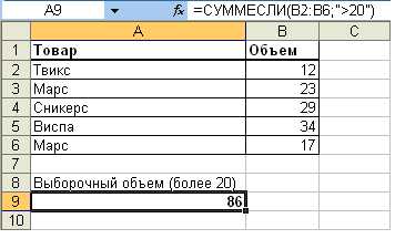
TO numerical functions conventionally include functions that calculate the quotient and remainder of division and round numbers.

1) calculation of the quotient and remainder. INTEGER function – rounds a number to the nearest lower integer. For example, INTEGER (5,7) – result 5; INTEGER (-5.7) – result 6. ROD function (number, divisor) – calculates the remainder of division by an integer.

2) rounding functions: ROUND (number, number_digits)

A) if number_digits is greater than 0, then the number is rounded to the specified number of decimal places to the right of the decimal separator;

B) if number_digits is 0, then the number is rounded to the nearest integer;

C) if number_digits is less than 0, then the number is rounded to the specified number of decimal places to the left of the decimal separator.

For example: Let the number 143.3184 be written in cell A4, then the ROUND (A4,2) formula will return the number 143.32. The formula ROUND(A4,0) will return the number 143. The formula ROUND(A4,-1) will return the number 140.

3) Slightly different problems are solved by the ROUNDUP (number, number_of_digits) and ROUNDUP (number, number_of_digits) functions. As their names suggest, they work like the ROUND function, but always round up or down.

4) The DROP function (number, number_digits) discards the fractional part of a number if the second argument is omitted. If you specify it, the function works as ROUND BOTTOM.

5) RAND function.

Returns a uniformly distributed random number greater than or equal to 0 and less than 1. A new random number is returned each time the worksheet is evaluated.

Syntax RAND()

Note:

To get a random real number between a and b, you can use the following formula:

RAND()*(b-a)+a

If you want to use the RAND function to generate a random number, but you don't want the number to change every time you calculate a cell value, you can type =RAND() in the formula bar and then press F9 to replace the formula with the random number.

Logic functions:

Some simple facts from mathematical logic.

For logical functions, arguments can take only two values: TRUE and FALSE. Therefore, logical functions can be specified as a table that lists all possible argument values and their corresponding function values.

AND and OR table

Table NOT

The NOT function can have only one argument, while the AND and OR functions can have two or more arguments.

In practice, logical expressions, as a rule, are not used “in their pure form.” A logical expression serves as the first argument of the IF function:

IF (logical_expression, value_if_true, value_if_false)

Boolean expressions are used to write conditions that compare numbers, functions, formulas, text, or Boolean values. Any logical expression must contain at least one comparison operator, which defines the relationship between the elements of the logical expression. Below is a list of Excel comparison operators

Equals

> More

< Меньше

>= Greater than or equal to

<= Меньше или равно

<>Not equal

The result of a logical expression is the logical value TRUE (1) or the logical value FALSE (0).

IF function

The IF function has the following syntax:

IF(logical_expression, value_if_true, value_if_false)

Formula =IF(A1>3,10,20) returns 10 if the value in cell A1 is greater than 3, and 20 otherwise:

You can use other functions as arguments to the IF function. The IF function can use text arguments. For example:=IF(A1>=4;"Passed the test","Failed the test").

You can use text arguments in the IF function so that if the condition is not met, it returns an empty string instead of 0. For example:=IF(SUM(A1:A3)=30,A10,"").

The boolean_expression argument of the IF function can contain a text value. For example:=IF(A1="Dynamo";10;290). This formula returns 10 if cell A1 contains the string "Dynamo" and 290 if it contains any other value. Match between compared text values must be accurate, but not case sensitive.

Functions AND, OR, NOT

Functions AND (AND), OR (OR), NOT (NOT) - allow you to create complex logical expressions. These functions work in conjunction with simple comparison operators. The AND and OR functions can have up to 30 Boolean arguments and have the syntax:

AND(boolean_value1;boolean_value2...)
=OR(boolean_value1, boolean_value2...)

The NOT function has only one argument and the following syntax:

NOT(boolean_value)

Arguments to the AND, OR, and NOT functions cannot be Boolean expressions, arrays, or cell references containing Boolean values.

Let's give an example. Let Excel return the text "Passed" if the student has a GPA greater than 4 (cell A2) and a class absence rate of less than 3 (cell A3). The formula will look like:=IF(AND(A2>4,A3<3);"Прошел";"Не прошел")

Even though the OR function has the same arguments as the AND function, the results are completely different. So, if in the previous formula we replace the AND function with OR, then the student will pass if at least one of the conditions is met (average score more than 4 or absenteeism less than 3). Thus, the OR function returns the logical value TRUE if at least one of the logical expressions is true, and the AND function returns the logical value TRUE only if all the logical expressions are true.

There are features of writing logical functions in table processors: first, the name of the logical function is written, and then the logical operands are listed in parentheses.

Let us assume that the student passed the session if the average exam score is more than 3 (cell A 2) and the number of absences is less than 10% (cell B 2). Otherwise, the student did not pass the session. The IF function implementing this algorithm would look like this:IF(AND(A2>3,B2<=10%);”СДАЛ”;”НЕ СДАЛ”).

The function does NOT reverse the value of its argument to the opposite boolean value and is usually used in combination with other functions. This function returns the logical value TRUE if the argument is FALSE and the logical value FALSE if the argument is TRUE.

Nested IF functions

Sometimes it can be very difficult to solve a logic problem using only comparison operators and AND, OR, NOT functions. In these cases, you can use nested IF functions.

Let's assume that three text constants can be entered into cell A1: “red”, “yellow”, “green”. Depending on the value of the text constant, it is necessary to implement the IF function, which issues the appropriate recommendations: “stop”, “wait”, “go”. The function will look like this:
IF(A1=”red”;”stop”;IF(A1=”yellow”;”wait”;”go”))

For example, the following formula uses three IF functions:=IF(A1=100,"Always";IF(AND(A1>=80;A1<100);"Обычно";

IF(AND(A1>=60,A1<80);"Иногда";"Никогда")))

If the value in cell A1 is an integer, the formula reads: "If the value in cell A1 is 100, return the string "Always." Otherwise, if the value in cell A1 is between 80 and 100, return "Usually." otherwise, if the value in cell A1 is between 60 and 80, return the row "Sometimes". AND, if none of these conditions are true, return the row "Never". A total of 7 levels of nesting of IF functions are allowed.

Functions TRUE and FALSE

The TRUE and FALSE functions provide an alternative way to write the Boolean values TRUE and FALSE. These functions have no arguments and look like this:

TRUE()
=FALSE()

For example, cell A1 contains a Boolean expression. Then the following function will return "Pass" if the expression in cell A1 evaluates to TRUE:

IF(A1=TRUE();"Pass";"Stop")

Otherwise, the formula will return "Stop".

Nested functions

In some cases it may be necessary to use a function as one of thearguments (Argument. Values used by a function to perform operations or calculations. The type of argument used by a function depends on the specific function. Typically, arguments used by functions are numbers, text, cell references, and names.)another function. For example, the following formula uses a nested AVERAGE function and compares the result to the value 50.

The AVERAGE and SUM functions are nested within the IF function.

Valid calculated value typesA nested function used as an argument must evaluate to the data type corresponding to that argument. For example, if the argument should be logical, i.e. have the value TRUE or FALSE, then the nested function as a result of calculations must also return the logical value either TRUE or FALSE. Otherwise, Microsoft Excel will generate the error “#VALUE!”

Limit number of function nesting levelsYou can use up to seven levels of nested functions in formulas. When function B is an argument to function A, function B is at the second level of nesting. For example, the AVERAGE and SUM functions are considered second-level functions because they are both arguments to the IF function. A function nested as an argument in the AVERAGE function will be a third-level function, and so on.

You can insert another function into one function. Up to 7 levels of nesting of functions are allowed (in Office 2007 - up to 64). Of course, the function can be written manually (write the name of the nested function, open parentheses, add semicolons). However, this contradicts the very ideology of the function wizard, which should facilitatewriting formulas, protecting the user from errors and minimizing manual work. There is a more convenient way to nest a function - a special button on the Formula Bar panel":

After selecting the desired function from the drop-down list, Excel will insert the function name and parentheses at the specified location in the formula (in the active argument text field). After this windowThe function wizard for the previous function (in this example "SUM") will change to the window for the function being inserted ("DEGREE"), and its name in the formula will become bold:

Switch to another function in a formula

To return to the window for the "SUM" function again, simply click on its name in the formula bar, and the window for the degree will change to the window for "SUM". After this, the “SUM” function in the name will become bold, indicating that the window is currently open for it.

Using names

You can name cells and ranges and then use them in formulas. Name is a word or string of characters that represents a cell, range of cells, formula, or constant. Names can be used on any sheet in the workbook.

Using names instead of links eliminates the need to enter complex cell references. Names defined in the current sheet can be used in any other sheets in the workbook. When specifying names, the following rules must be observed:

the name can begin with a letter, a backslash (\) or an underscore;
- Only letters, numbers, backslashes and underscores can be used in the name;
- you cannot use names that are interpreted as references to cells and single letters R and C;
- To define a name, you need to select a cell or range and use the menu command Insert  Name  Assign , and then enter the user-selected name in the “Name” field;
- To insert a name into a formula, use the menu command Insert  Name  Insert and then the appropriate name is selected from the list.

Naming

You can assign a name to a cell or range of cells.

Select a cell or range of cells.
In Group Specific names On the Formulas tab, click the Assign Name button.
In the Create a name window, in the Name field enter a cell or range name ( rice. 6.18).

Rice. 6.18. Naming a cell

To set the scope of a name in a combo box Region select Book or the name of a sheet in a workbook.
If desired, in the field Note you can enter a note about the name, which will then be displayed in the window Name Manager.

For ease of use, it is recommended to create names that are short and memorable. The first character in the name must be a letter or an underscore. Other characters in the name can be letters, numbers, periods, and underscores. Spaces are not allowed. Also not allowed are names that have the same appearance as cell references, for example Z$100 or R1C1 . A name can have more than one word. Underscores and periods can be used as word separators, for example: Year_2007 or Year.2007 . The name can contain up to 255 characters. The name can consist of lowercase and uppercase letters, but Excel does not distinguish between them.

When working in Excel You can link to other sheets in the same workbook. For example, to enter into a cell A 3 sheets Sheet 1 cell reference A 1 sheet Sheet2, you should perform the following sequence of actions:

select cell A 3 on sheet Sheet1 and enter an equal sign;
click on the Sheet2 shortcut at the bottom of the workbook window;
click on a cell A 1 and press the key< Enter > . After this, the sheet Sheet1 will be activated again and in the cell A 3 the formula appears =Sheet2! A 1.

When using references to cells of other sheets and books in the formulas you create, during the process of creating a formula, you should go to another sheet of the current workbook or to another book and select the required cell there.

Each time you move to another sheet, its name is automatically added to the cell reference. The sheet name and cell address are separated by a service character! (Exclamation point).

For example, in a formula in a cell D2 in the table in Fig. 6.13 cell used A4 sheet Course of the current book.

You can similarly reference cells that are in another workbook. For example, cell reference A 1 sheet Sheet1 of the book Book2 has the following form: =[Book2]Sheet1!$ A $1. By default, when you create a link to cells that belong to another workbook, E x cel inserts an absolute link.

2.12. Conditional Formatting

Excel 2007 provides even more powerful and convenient conditional formatting tools.

This formatting is convenient for data analysis - you can color the worksheet so that each color corresponds to specific data. In this case, even a quick glance at a sheet of document will be enough to assess problem areas.

To apply conditional formatting, use the button"Conditional Formatting" in the Styles panel of the Home ribbon.

To better understand how conditional formatting works, select a group of cells with data already entered, click the button"Conditional Formatting"and see the different formatting options.

By default, the program automatically determines the minimum and maximum values in the selected range and then formats them in equal percentages.

To extend conditional formatting to other cells, you need to right-click the lower right corner of the newly formatted cell and select the item in the context menu"Fill in formats only".

To remove conditional formatting, select the desired range of cells and click"Conditional Formatting" and select item "Delete rules".

Open computer science lesson in 9th grade
Logical functions in MS EXCEL spreadsheets

The purpose of the lesson: study the logical functions of MS Excel used in solving problems.

Educational objectives of the lesson:

explore functions AND, OR, IF from category Use the function wizard to select from a category;

learn to use them when solving problems.

Planned results:

Subject: know and apply functions AND, OR, IF from category Use the function wizard to select from a category when solving problems.

Metasubject:

Regulatory: independently formulate goals, objectives, lesson problems, and plan activities.

Cognitive: analyze, establish cause-and-effect relationships, conduct a comprehensive search for information in sources of various types to solve problems, compare.

Communicative: collaborate with the teacher, classmates, express their own point of view; construct understandable speech statements.

Personal: instill interest in the subject, topic, apply the acquired knowledge in various areas of educational activity.

Will learn: use built-in functions, apply logical functions.

Lesson type: combined

Equipment: multimedia projector, laptops; software: MSExcel.

Forms of student work: frontal, group, individual

Used T technologies:

problem-based learning;

development of critical thinking;

systemic and activity-based technological approach to learning;

information Technology

flipped classroom model

DURING THE CLASSES

1. Organizational moment - less than 1 minute. Greets students. Conducts n checking readiness for the lesson.

Hello, very glad to see you again!

2. Updating knowledge – 10 min.(d/z check – “flipped classroom” model) .

Self-assessment sheet. In order to gain full knowledge, it is important to record how successful our lesson will be. This self-assessment sheet will give you the opportunity to record every detail of your work throughout the lesson as you study the topic.

If you are satisfied (coped it), satisfied (partially), disappointed (didn’t understand, couldn’t) with how our lesson went, then mark your attitude towards the elements of the lesson in the appropriate cell on the sheet (Annex 1).

We continue to study the topic related toinformation technology software, namely the Excel spreadsheet application environment.

Frontal survey to update technological knowledge in the environment http://learningapps.org/( LearningApps.org is a Web 2.0 application to support learning and teaching through interactive modules ) .

1. You are offered a task Vlearningapps.org environment: (individual work on computers). Get started!

This task takes 1 minute.

http://learningapps.org/watch?v=poc2tgjqa16

Now let's check the task together (the student is called to the board)

Function AndPurpose .

Mathematical orStatistical) (print on sheets of paper or on the interactive whiteboard).Appendix 2.

	Purpose

	Calculating the square root

SUM, SQRT, SIN - Mathematical

MIN, AVERAGE, - Statistical

Let's compare your answers with the correct result (on the screen ). Appendix 2. Answers

3. Now please look at the screen. You are presented with a task ( Demo version 2013, task No. 19 ).

Discussion with the whole class.

1. How do you think about solving a problem with data in 1000 rows of a table? (autocopy formula)

2. Let's think about what formula you can set if you need to calculate total transportation distance fromOctober 1st to 3rd ? The answer must be written in cell H2 of the table.

=SUM(D2:D118)

=AVERAGEIF(B2:B371,"Sticky";F2:F371)

Well done! We did it!

Slide 1. Table

3. Motivation (problem formulation) – 10-12 min.

At home you watched a video (You can have a presentation with detailed comments, which replaces the teacher’s explanation in the video ).

Based on this video, formulate the topic of the lesson ( ), state the purpose of our lesson (know and in MS Excel ).

Slide 2. Table

WHAT WE ALREADY KNOW	WHAT WILL WE LEARN IN TODAY'S LESSON?


	Apply logical functions to solve problems
	Logic functions

Appendix 3.Problem: On your desk in front of you is a card with a task. Can we solve this problem?

Work in groups.

Group 1: Solve the problem of using the functions AND, OR (on sheets of paper).

__________________________________________________________________________________________________________________________________________________________

Excel Excel → Task_group 1).

After discussion, we come to the conclusion that the formula should be entered in cell D4 =And(B4-C4=C4*0.07). In other words, we used a logical function with one condition - ensuring sales exceed the plan by 7%.

Tell me, in this problem, is it possible to use the OR function for the same purpose?

It is possible, with one condition, to receive the answers “true” or “false” in the cell.

Group 2: Solve the problem of using the IF function (on sheets of paper).

1. Determine and enter a formula with a logical function so that the entry “accepted” or “not accepted” appears opposite the last name of each boy or girl in the Choice column.

The spreadsheet field looks like this:

2.Formulate a conclusion (analysis of the logical functions used):

______________________________________________________________________________________________________________________________________________________________________

3.Check this problem by solving it inExcel .(The file is located on the Desktop → folderExcel → Task_group 2).

Solution: “Dance School” enter the formula in cell D6:=IF(AND(AND(B6=168,B6

Show ready-made solutions to problems (highlight them on the screen). Discussion of tasks. Did you manage to solve the problem posed to you?

Well done! Now let's e Let's check this problem by solving it inExcel .

4. Primary consolidation of the material (practical part) – 15 -17 min.

Work in groups on the computer. Role-playing game.

Students are divided into three groups of 5-6 people. Each group will represent one of the organizations: “ Svyaztelekom», « SuperBukh», « Chance».

The groups are given signs with the names of organizations, cards with tasks (client requests), and are allocated one computer each ( Applications No. 4).

The organization enters information into prepared tables and prepares the result (a report to the manager; the report must be beautifully and effectively formatted; the teacher acts as the manager).

In groups, a senior director is selected - the director of the organization, who manages the work of the group and must organize it so that each participant performs his task: one works on the computer with a spreadsheet (operator), the second prepares a report on the work of the group (secretary), the third checks the correctness of the mathematical calculations (accountant).

If working on a task is difficult, groups can get help from a teacher.

The role-playing game lasts 10 minutes. Then, for 5 minutes, the groups talk about their work - present their spreadsheet, describe difficulties and successes in their work, and carry out self-assessment.

Organization " Svyaztelekom» helps the subscriber calculate how much each person should pay for telephone calls.

Task "Cost calculation telephone negotiations"

Five subscribers call from city A to city B. If a long-distance telephone call was made on weekends (Saturday, Sunday), or on holidays, or on weekdays from 20 pm to 8 am, then it is calculated at a reduced rate with 50% discount, no benefits at other times. Calculate how much each of the five subscribers must pay for negotiations.

Solution

We use a pre-prepared table of the cost of telephone calls.

If the call is made at a reduced rate, then the following condition must be met: Day of the week = “Saturday” OR Day of the week = “Sunday” OR Holiday “Yes” OR start time of negotiations = 20 OR Start time of negotiations G3 enter the formula: IF (OR (C3= “Saturday”; C3= “Sunday”; D3= “Yes”; E3=20; E3

Organization " SuperBukh» helps the store discounts

Task “Discount”. discountsdiscounts: buyer, purchase price,discount, purchase price includingdiscountsdiscount, the cost of which exceeds k rubles.

Solution:

We prepare a table in the form:

We enter the corresponding data in cells A1:B7.

In cell C2 we enter the formula =B2*0.1 (since discount for a purchase of 10%, then the initial purchase price must be multiplied by 0.1).

In cell D2 we enter the formula =B2-C2 (since we calculate the cost taking into account discounts)

In cell E2, enter the formula =IF(B2=$B$9;D2;B2). In this formula, you need to pay attention to the absolute reference to cell B9.

When entering a formula into cell E2, we encountered a situation where, when inserting the built-in IF function, we need to make a reference to a cell as the value of a logical expression.

Organization " Chance» helps companies

Task "Debt"

1. Find employees who simultaneously have debts on a consumer loan and a loan for housing construction, and withhold 20% of the amount accrued to them.

Solution: For our example, the logical function will look like this:

=IF(AND (C30,D30); VZ*0.2; "-")

This logical function means the following: if at the same time the debt on a consumer loan and a loan for housing construction is greater than zero, then it is necessary to withhold 20% of the accrued amount, otherwise it is necessary to display the gaps.

2. Find employees who simultaneously have debts on both types of loans, and withhold 20% of the amount accrued to them to repay the loans. From other employees who have debt on any one type of loan, 10% of the amount accrued to them is withheld. For employees who do not have loan debt, enter “b/c” in the “Withheld” column.

Solution:

In our example, the logical function will look like this:

=IF (AND(C30;D30);B3*0.2;IF (AND (C3=0;D3=0);"b/k"; VZ*0.1))

are equal to zero, then it is necessary to withdraw “b/c”, otherwise it is necessary to withhold 10% of the accrued amount.

Completion of practical work.

5. Physical education (1 min) for the eyes and back. Conducted by a student!(Can be done as a survey on the topic: TRIZ “Yes-NO” technique, if you agree - YES stand up (NO - sit down) or any other movement, you can change the movements on each question)

Without getting up from your desk, take a comfortable position - your back is straight, your eyes are open, your gaze is directed straight. The exercises must be performed easily without tension.

1. Changing the focal length: look at the tip of the nose, then into the distance. Look at the tip of a finger or pencil held at a distance of 30 cm from the eyes, then into the distance.

Repeat several times.

2. Squeeze your eyelids, then blink several times.

3. We remove the load from the muscles involved in the movement of the eyeball: look to the left - straight, to the right - straight, without delay in the abducted position.

4. Circular eye movements - from 1 to 10 circles to the left and right. First quickly, then as slowly as possible.

5. You need to finish the gymnastics by massaging your eyelids, gently stroking them with your index and middle fingers in the direction from the nose to the temples, and then rub your palms lightly. Without effort, cover your closed eyes with them to completely block them from the light (for 1 minute). Imagine being plunged into complete darkness.

Thank you!

6. Checking the assimilation of new material usingMyTest (individual) – 2 min.

You are asked to answer the test questions, the system will analyze the answers and display the result. Upon completion, you will enter the result on the Self-Assessment Sheet.

The test is located on the Desktop → Testing → Logical functions inMS Excel .

A)The dance school accepts girls and boys with a height of no less than 168 cm and no higher than 178 cm.

Possible answers:

1. OR (Height168; Height

2. I (Height 168)

3. And (Height =168)

b) The dance school accepts girls and boys with a height of no less than 168 cm and no higher than 178 cm. The weight of those entering the dance school must be correlated with height using the formula: weight value

Possible answers:

1. AND(OR (Height168; HeightRost - 115))

2. And(And (Height=168; Height Height - 115))

3. AND(OR (Height=168; HeightHeight - 115))

V) In the range from A2 to A32 are the daily temperature values for the month of December. It is considered an anomaly if the average monthly temperature goes beyond -30 to +10. Is the temperature abnormal?

Possible answers:

1. AND (AVERAGE(A2:A32)=10; AVERAGE(A2:A32)

2. AND (AVERAGE(A2:A32)=-30)

3. OR (AVERAGE(A2:A32)=10; AVERAGE(A2:A32)

G)What logical expression corresponds to the double inequality 0

1. I(A10; A1

d)What logical expression corresponds to the condition “children under 12 years old or old people over 70 years old.”

1. OR(children=70)

2. IF (OR(children=70)

3. I(children=70)

e)For a given value X, you need to calculate the value Y using one of the formulas: if x5, then y:=x-8, otherwise y:=x+3. What the formula will look like:

Possible answers:

1. =IF(B15;B 1-8; B 1+3)

2. =IF(AND(B15;B 1-8;B 1+3))

3. =IF(OR(B15,B 1-8,B 1+3))

7. Summing up the lesson – 5 min.

What goals did we set for ourselves at the beginning of the lesson?

What new did you learn?

What have you learned?

After discussionon the screen:

WHAT WE ALREADY KNOW	WHAT WILL WE LEARN IN TODAY'S LESSON?	WHAT WE CAN, WHAT WE LEARNED
The contents of the ET cell can be text, number and formula	What logical functions are there in spreadsheets (MSExcel)?	The logical functions AND, OR implement the corresponding logical operations. The logical IF function allows you to select an action depending on the condition (logical expression).
	Rules for entering logical functions in spreadsheets (MSExcel)?
	Apply logical functions to solve problems
Mathematical, statistical functions	Logic functions

8. Homework 1 min .:

Our lesson has come to an end. You worked well in groups, successfully completed tasks individually, I am pleased with you. Thank you!

The knowledge gained today in the lesson will allow you to solve calculation problems of various levels in a spreadsheet in various areas of human activity, predict the result and make an analysis.

There are sheets of paper on your desksAppendix No. 5 - this is homework, using the reference notes, knowledge gained in class, solve the problem using logical functions.

Appendix No. 5

Task 1.

Task 2.

WHAT WE ALREADY KNOW	WHAT WILL WE LEARN IN TODAY'S LESSON?	WHAT WE CAN, WHAT WE LEARNED
The contents of the ET cell can be text, number and formula	What logical functions are there in spreadsheets (MSExcel)?
	Rules for entering logical functions in spreadsheets (MSExcel)?	Rules for entering logical functions into ET
	Apply logical functions to solve problems	Use MSExcel logical functions to solve problems
Mathematical, statistical functions	Logic functions

And I would like to finish the lessonFrench scientist Gustav Guillaume: Epigraph on the presentation slide: “The road can be mastered by those who walk, but computer science by those who think.”

Goodbye!

"Appendix 1. Self-assessment sheet"

Self-assessment sheet for 9th grade student(s) FI_________________________________

1. Criteria

Thematic control of knowledge.

POINTS

2. Criteria.

Determining the topic, purpose, problem of the lesson

POINTS

3.Criteria

Work in groups.

Working with reference notes (semantic viewing of a video, searching for information)

POINTS

4. Criteria

Primary assimilation of subject knowledge.

Work in groups on the computer Role-playing game.

POINTS

All (4 parts)

Partially (3 parts)

Couldn't (2 parts)

Myself

with the help of a teacher

I couldn't

All by myself

Partially

I couldn't

All

Partially

I couldn't

1. Exercise: bring the correct parts together so that they are “glued together” with tape

1. I have determined the topic of the lesson.

1.I entered the formula

1.I completed the task correctly (practical work on the computer)

2. Established a correspondence, entered the function category

All (5)

Partially(4-3)

Couldn't (2-0)

2. I formulated the purpose of the lesson

2.I formulated a conclusion

All by myself

Partially

I couldn't

2. Managed to cope with the assigned role

Yes

Partially

3. Solved the problem

All (2 tasks)

Partially (1 task)

I couldn't (not a single task)

3. I understood the task (problem) assigned to me

3. I checked the problem by solving it in MS Excel

Yes, completely

Partially

I couldn't

3. Describe difficulties and successes in your work

Myself

With everyone

I couldn't

5.Criteria

Testing the assimilation of new material using MyTest (individual)

POINTS

My total points: ________ Mark: ________

Evaluation criteria:

“5” - 26 – 20 points

“4” - 19–15 points

“3” - 14–10 points

Less than 10 points. Dont be upset! We still need to study.

Yes, completely

Partially

I couldn't

1.I solved the test correctly (I succeeded)

View document contents
"Appendix 2. Compliance task"

Appendix No. 2

1.Match the correspondence betweenFunction AndPurpose .

Function	Purpose
	Calculate the sum of values in a given range
	Calculating the square root
	Calculating a trigonometric function
	Calculate the minimum value within a given range
	Calculates the arithmetic mean of a range of arguments

2. Enter the function category (Mathematical orStatistical ).

View document contents
“Appendix 3. Problem. Assignment on sheets for groups”

Appendix No. 3

1st group:

SOLVE THE PROBLEM ON APPLYING FUNCTIONS AND, OR

You are faced with the task of paying bonuses for increasing the number of sales to company employees by more than 7%.

The spreadsheet field looks like this:

1. Enter a formula so that column D displays TRUE for the employee who should receive a bonus and FALSE for the employee who should not receive a bonus?

2.Formulate a conclusion (analysis of the logical functions used):

____________________________________________________________________________________________________________________________________________________________________________________

3.Check this problem by solving it inExcel .

(The file is located on the Desktop → folderExcel → Task_ group 1).

Group 2:

SOLVE THE PROBLEM ON USING THE IF FUNCTION

Determine and enter a formula with a logical function so that the entry “accepted” or “not accepted” appears opposite the last name of each boy or girl in the Choice column.

The spreadsheet field looks like this:

Formulate a conclusion (analysis of the logical functions used):

_______________________________________________________________________________________________________________________________________________________________________________________

Check this problem by solving it inExcel .

(The file is located on the Desktop → folderExcel → Task_ group 2).

View document contents
"Appendix 4. Role-playing game"

Appendix No. 4

Organization " SVIAZTELECOM» helps the subscriber calculate

how much each person has to pay

for telephone conversations.

Task “CALCULATING THE COST TELEPHONE NEGOTIATIONS"

Five subscribers call from city A to city B. Iftelephone a long-distance call was made on weekends (Saturday, Sunday), or on holidays, or on weekdays from 20 pm to 8 am, then it is calculated at a reduced rate with discount50%, no benefits at other times. Calculate how much each of the five subscribers must pay for negotiations.

__________________________________________________________________________________________________________________________________________________________________________________________________________________________________________________________________________________________________________________________________________________________________________________________________________________________________________________________________________________________________________

Organization " SuperBukh»

helps the store draw up a statement taking into accountdiscounts: buyer, purchase price,discount, purchase price includingdiscounts. And show which customers made purchases withdiscount, the cost of which exceeds k rubles.

Task “DISCOUNT”

Store customers enjoy 10% discounts, if the purchase price exceeds k rubles. Prepare a statement that takes into account discounts: buyer, purchase price, discount, purchase price including discounts. Make a table and show which customers made purchases with discount, the cost of which exceeds k rubles.

The organization enters information into prepared tables and prepares the result (a report to the manager; the report must be beautifully and effectively formatted (either in MS Excel or MS Word); the teacher acts as the manager).

In groups, choose a senior director of the organization, who will lead the work of the group and must organize it so that each participant performs his task: one works on the computer with a spreadsheet (operator), the second prepares a report on the work of the group (secretary), the third checks the accuracy mathematical calculations (accountant).

Execution time - 10 min. Then, for 5 minutes, the groups talk about their work - present their spreadsheet, describe difficulties and successes in their work.

DESCRIPTION OF DIFFICULTIES AND SUCCESSES IN WORK

Organization " CHANCE» helps companies find workers who have debt on a consumer loan and (or) a loan for housing construction, withhold % of the amount accrued to them.

Task "DEBT"

1. Find employees who simultaneously have debts on a consumer loan and a loan for housing construction, and withhold 20% of the amount accrued to them.

2. Find employees who simultaneously have debts on both types of loans, and withhold 20% of the amount accrued to them to repay the loans (Fig. 3). From other employees who have debt on any one type of loan, 10% of the amount accrued to them is withheld. For employees who do not have loan debt, enter in the "Withheld" column - "b/c ".

Execution time - 10 min. Then, for 5 minutes, the groups talk about their work - present their spreadsheet, describe difficulties and successes in their work.

DESCRIPTION OF DIFFICULTIES AND SUCCESSES IN WORK

View document contents
"Appendix 5. Homework"

Appendix No. 5

TASK 1.

The electricity supply company charges customers at a rate of k rubles per 1 kW/h and m rubles for each kw/h above the norm, which is 50 kw/h. The company's services are used by 10 clients. Calculate the fee for each client.

TASK 2.

10 all-round athletes take part in competitions in 5 sports. For each sport, an athlete scores a certain number of points. An athlete is awarded the title of master if he scores at least k points in total. How many athletes received the title of master?

"Logical Functions in Excel"

LOGICAL FUNCTIONS IN EXCEL

EXAMPLES OF THEIR APPLICATION

Simple IF function

Logical function " IF» is used to check conditions when performing calculations.

General function format:

IF(Logical_expression; value_if_true; value_if_false)

A Boolean expression is a condition.

If the condition is met, then the middle part of the expression comes into force, that is, “ value_if_true ».

If the condition is not met, then “ value_if_false ».

Simple IF function

Operation of the logical function " IF» is illustrated by the following

block diagram:

IF (condition; Operator1; Operator2)

2;”Pass”;”No pass”) B2 – address of the cell where the first student’s grade is located" width="640"

Task No. 1:

Let's create a spreadsheet like this:

In the column " Note 1"You should enter the formula so that the message " Test", if the score is greater than "2" and the message " No credit" otherwise.

Answer:

If (B22;”Pass”;”No pass”)

Difficult conditions

When solving many problems, they can be used as a logical expression difficult conditions.

Complex conditions consist of simple ones and are interconnected by the logical function “ AND"or logical function " OR ».

Logical OR function

General function format:

OR (Boolean_value_1;Boolean_value_2;......)

true"if at least one Boolean value is satisfied.

Task No. 2:

In the column " Note 2 Test", if the score is "3", "4" or "5" and the message " No credit" otherwise.

Answer:

If (OR(B2=3;B2=4;B2=5);”Pass”;”No pass”)

B2 – address of the cell where the first student’s grade is located

Logic AND function

General function format:

AND (Boolean_value_1;Boolean_value_2;......)

This logical expression (condition) takes the value " true" if all specified Boolean values are executed simultaneously. If at least one condition is not met, the value “ lie ».

2;B2 B2 – address of the cell where the first student’s grade is located" width="640"

Task No. 3:

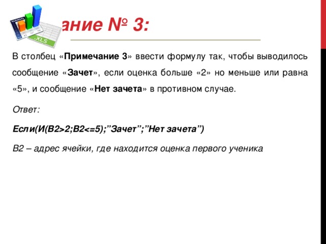
In the column " Note 3"Enter the formula so that the message " Test" if the score is greater than "2" but less than or equal to "5", and the message " No credit" otherwise.

Answer:

If(And(B22,B2

B2 – address of the cell where the first student’s grade is located

Nested IF Functions

Conditional statements can be nested when in the " Yes"(see block diagram Fig. 1) instead of operator 1 or in the branch " No" instead of operator 2 One more condition must be checked. In this case, use nested statements .

Let's consider the case when instead of operator 1 it is necessary to put one more condition. In this case, the block diagram looks like:

The logical function looks like:

IF(condition1; If (condition2; operator1; operator2); operator3)

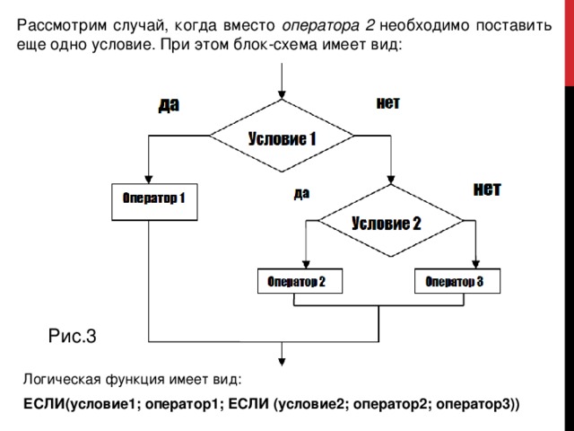
Let's consider the case when, instead of operator 2 One more condition must be set. In this case, the block diagram looks like:

The logical function looks like:

IF(condition1; operator1; IF(condition2; operator2; operator3))

2;B2" width="640"

Task No. 4:

In the column " Note 4"enter the formula so that the message " Test", if the score is "3", "4" or "5", the message " No credit Error" otherwise.

Answer:

If(OR(B2=3;B2=4;B2=5);”Credit”;If(OR(B2=1;B2=2);”No credit”;”Error”))

B2 – address of the cell where the first student’s grade is located

Another possible solution:

Answer:

If(And(B22,B2

Task No. 5:

In the column " Note 5"enter the formula so that the message " Great", if the rating is "5", the message " Fine", if the score is "4", the message " Satisfactorily", if the score is 3, the message " Unsatisfactory" or " Badly", if the score is "2" or "1", and the message " Error" otherwise.

Answer:

If(B2=3;”Satisfactory”;If(B2=4;”Good”;If(B2=5;”Excellent”;If(OR(B2=1;B2=2); “Unsatisfactory”; “Error” ))))

B2 – address of the cell where the first student’s grade is located

View presentation content
"Table"

MS EXCEL

WHAT WE ALREADY KNOW

The contents of the ET cell can be text, number and formula

Mathematical, statistical functions

MS EXCEL

WHAT WE ALREADY KNOW

WHAT WILL WE LEARN IN TODAY'S LESSON?

The contents of the ET cell can be text, number and formula

Apply logical functions to solve problems

Mathematical, statistical functions

Logic functions

MS EXCEL

The contents of the ET cell can be text, number and formula

WHAT WE ALREADY KNOW

WHAT WILL WE LEARN IN TODAY'S LESSON?

What logical functions are there in spreadsheets (MS Excel)?

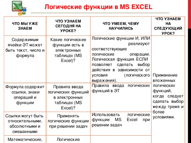
WHAT WE CAN, WHAT WE LEARNED

Logical functions AND, OR implement the corresponding logical operations. The logical IF function allows you to select an action depending on a condition (logical expression).

Rules for entering logical functions in spreadsheets (MS Excel)?

Rules for entering logical functions into ET

Apply logical functions to solve problems

Mathematical, statistical functions

Logic functions

Logical functions in MS EXCEL

WHAT WE ALREADY KNOW

The contents of the ET cell can be text, number and formula

WHAT WILL WE LEARN IN TODAY'S LESSON?

What logical functions are there in spreadsheets (MS Excel)?

WHAT WE CAN, WHAT WE LEARNED

WHAT WILL WE LEARN FOR THE NEXT LESSON?

Rules for entering logical functions in spreadsheets (MS Excel)?

Logical functions AND, OR implement the corresponding logical operations. The logical IF function allows you to select an action depending on a condition (logical expression).

Mathematical, statistical functions

Apply logical functions to solve problems

Rules for entering logical functions into ET

Logic functions

Use logical functions of MS Excel when solving problems

The use of nested logical functions when a choice must be made between three or more conditions.