Extract all repetitions of the desired value example. We escape from routine work using the VLOOKUP function in Excel.
Excel is popular due to its accessibility and simplicity, as it does not require special knowledge and skills. Tabular view the provision of information is understandable to any user, and a wide range of “Wizard functions”, which allows you to carry out any manipulations and calculations with the provided data.
One of the widely known Excel formulas is vertical viewing. Usage VLOOKUP functions At first glance it seems quite complicated, but this is only at first.
How Excel VLOOKUP works
When working with the VLOOKUP formula, keep in mind that it searches for the desired value exclusively in columns, and not in rows. To use the function, a minimum number of columns is required - two, no maximum.
The VLOOKUP function searches for a given criterion, which can have any format (text, numeric, monetary, date and time, etc.) in the table. If a record is found, it produces (substitutes) the value entered in the same line, but from the desired table column, that is, the corresponding given criterion. If the required value is not found, then the error #N/A is issued (in the English version #N/A).
Need for use
The VLOOKUP function comes to the aid of the operator when he needs to quickly find and apply it in further calculations, analysis or forecast. specific value from the table large sizes. The main thing when using this formula is to ensure that the specified search area is selected correctly. It should include all records, that is, from the first to the last.
The most common use of VLOOKUP is to compare or add data in two tables using a certain criterion. Moreover, search ranges can be large and contain thousands of fields, located on different sheets or books.
The VLOOKUP function is shown, how to use it, how to carry out calculations, as an example in the figure above. Here is a table of retail sales sizes depending on the region and manager. The search criterion is a specific manager (his first and last name), and the desired value is the amount of his sales.
As a result of the VLOOKUP function, a new table, in which the specific manager you are looking for is quickly matched with his sales amount.
Algorithm for filling out the formula
The VLOOKUP formula is located in the "Function Wizard" tab and the "Links and Arrays" section. The function dialog box looks like this: 
Arguments are entered into the formula in order:
- The desired value is what the function must find, and the options for which are the values of the cell, its address, the name given to it by the operator. In our case, this is the manager’s last and first name.
- Table - a range of rows and columns in which the criterion is searched.
- The column number is its ordinal number in which the sales amount is located, that is, the result of the formula.
- Interval viewing. It holds the value either FALSE or TRUE. Moreover, FALSE only returns exact match, TRUE - allows searching for an approximate value.
Example of using the function
Function VLOOKUP example may have the following uses: when conducting business in a commercial enterprise in Excel tables column A contains the name of the product, and column B contains the corresponding price. To create a proposal, in column C you need to find the cost for a certain product, which you want to display in column D.
The formula written in D will look like this: =VLOOKUP (C1; A1:B5; 2; 0), that is, =VLOOKUP (search value; table data range; column serial number; 0). FALSE can be used as the fourth argument instead of 0.
To fill out the proposal table, the resulting formula must be copied to the entire column D.
You can freeze the working data range area using absolute references. To do this, $ signs are manually placed in front of the alphabetic and numerical values of the addresses of the leftmost and rightmost cells of the table. In our case, the formula takes the form: =VPR (C1; $A$1:$B$5; 2; 0).
Errors during use
The VLOOKUP function does not work and then an error message appears in the result output column (#N/A or #N/A). This happens in the following cases:
- The formula has been entered, but the required criteria column is not filled in (in in this case column C).
- Column C contains a value that is not in column A (in the data search range). To check the presence of the desired value, select the criteria column and in the menu tab "Edit" - "Find" insert this entry, start the search. If the program does not find it, then it is missing.
- The formats of the cells of columns A and C (the search criteria) are different, for example, one has a text format, and the other has a numeric one. You can change the cell format by going to cell editing (F2). Such problems usually arise when importing data from other application programs. To avoid this kind of errors in VPR formula It is possible to embed the following functions: VALUE or TEXT. Execution of these algorithms automatically converts the cell format.
- The function code contains unprintable characters or spaces. Then you should carefully check the formula for input errors.
- Set rough search, that is, the fourth argument of the VLOOKUP function is 1 or TRUE, and the table is not sorted by ascending value. In this case, the search criteria column needs to be sorted in ascending order.
Moreover, when organizing a new pivot table the specified search criteria can be in any order and sequence and do not necessarily fit full list(partial sample).
Features of use as timelapse 1 or TRUE
Error number 5 is quite common and is clearly depicted in the figure below.
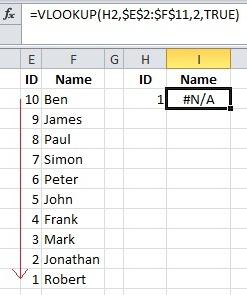
IN in this example the list of names according to numbering is sorted not in ascending order, but in descending order. Moreover, (1) was used as an interval scan, which immediately interrupts the search when a value greater than the desired value is detected, so an error is generated.
When using 1 or TRUE in the fourth argument, you must ensure that the column with the criteria you are looking for is sorted in ascending order. When using 0 or FALSE this need disappears, but then there is also no possibility of interval viewing.
Just keep in mind that it is especially important to sort interval tables. Otherwise, the VLOOKUP function will display incorrect data in the cells.
Other nuances when working with the VLOOKUP function
To make it easier to work with such a formula, you can title the range of the table in which the search is carried out (the second argument), as shown in the figure.

In this case, the sales table area is titled. To do this, select the table, excluding the column headers, and assign a name to it in the name field (on the left under the tab bar).
Another option - to title - involves selecting a range of data, then going to the menu "Insert" - "Name" - "Assign".
To use data located on another sheet workbook, using the VLOOKUP function, you need to specify the location of the data range in the second argument of the formula. For example, =VLOOKUP 2; 0), where is Sheet2! - is a link to the required worksheet, and $A$1:$B$5 is the address of the data search range.
An example of organizing the educational process with VPR
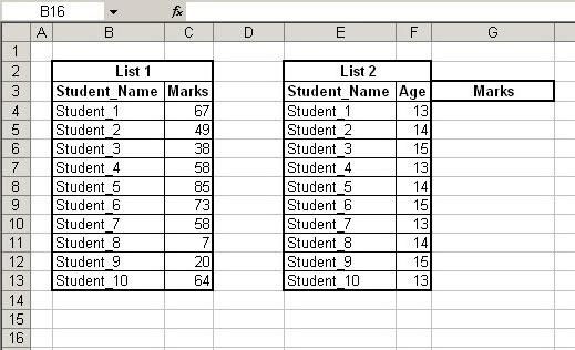
Quite convenient in Excel VLOOKUP function be used not only by trading firms, but also by educational institutions to optimize the process of comparing pupils (students) with their grades. Examples of these tasks are shown in the figures below.
There are two tables with lists of students. One with their ratings, the second indicates their age. It is necessary to compare both tables so that their grades are displayed along with the age of the students, that is, enter an additional column in the second list.
The VLOOKUP function does an excellent job of solving this problem. In column G under the heading “Evaluations” the corresponding formula is written: =VPR (E4, B3:C13, 2, 0). It needs to be copied to the entire table column.
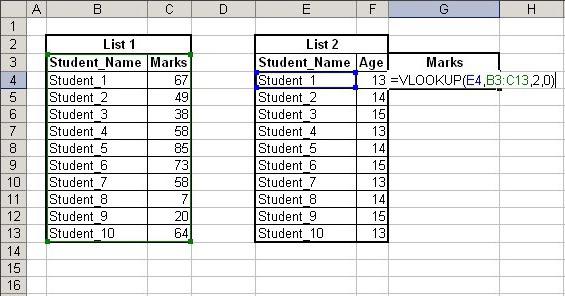
As a result of execution, the VLOOKUP function will display the grades received by certain students.
An example of organizing a search system with VLOOKUP
Another example of using the VLOOKUP function is the organization of a search system, when in the database, according to a given criterion, the corresponding value should be found. So, the figure shows a list with the names of animals and their belonging to a specific species.
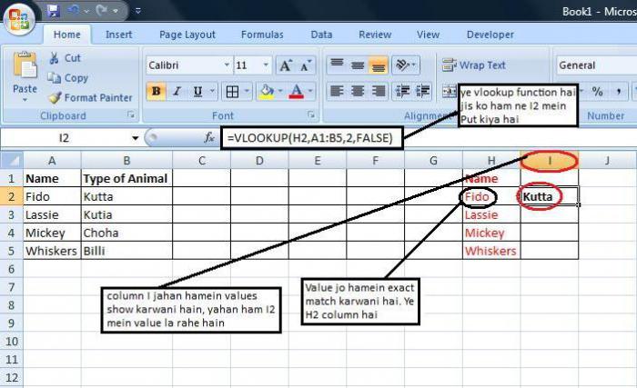
At VPR help a new table is created in which it is easy to find its species by the name of the animal. Similar ones are relevant search engines when working with large lists. In order not to manually review all records, you can quickly use the search and get the desired result.
The VLOOKUP (Vertical Lookup) function searches a table of data and, based on the search query criteria, returns the corresponding value from a specific column. Very often it is necessary to use several conditions at once in a search query. But by default this function cannot handle more than one condition. Therefore, you should use a very simple formula that will expand the capabilities of the VLOOKUP function across several columns at the same time.
Operation of the VLOOKUP function according to several criteria
For clarity, let’s analyze the VLOOKUP formula with an example of several conditions. As an example, we will use a schematic report on the revenue of sales representatives for the quarter:
In this report, you need to find the revenue figure for a specific sales representative on a specific date. Considering the search conditions, our request must contain 2 conditions:
- – Date of delivery of proceeds to the cashier.
- – Last name of the sales representative.
To solve this problem, we will use the VLOOKUP function under several conditions and create the following formula:
- In cell C1, enter the first value for the first criterion search query. For example, date: 03/22/2017.
- In cell C2, enter the last name of the sales representative (for example, Novikov). This value will be used as the second argument of the search query.
- In cell C3 we will receive the search result; to do this, enter the formula there:
- After entering the formula, press the hotkey combination CTRL+SHIFT+Enter to confirm, since the formula must be executed in an array.
The result of a search in the table using two conditions:
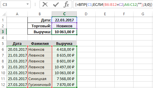
The amount of revenue of a specific sales representative on a specific date was found.
Analysis of the principle of operation of the formula for the VLOOKUP function with several conditions:
The first argument of the =VLOOKUP() function is the first condition for searching for a value in the sales representatives revenue report table. The second argument contains a virtual table created as a result of a massive calculation logical function=IF(). Each last name in the range of cells B6:B12 is compared with the value in cell C2. Thus, a conditional data array is created in memory with elements of the TRUE and FALSE values.
Then, thanks to the formula, in the program memory each true element is replaced by a 3-element data set:
- element – Date.
- element – Last name.
- element – Revenue.
And each false element in memory is replaced with a 3-element set of empty ones text values(""). As a result, a new table is created in the program memory, with which the VLOOKUP function will already work. It ignores all empty element datasets. And non-empty elements are matched to the value of cell C1, which was used as the first criterion of the search query (Date). In short, the table in memory is checked by the VLOOKUP function with one search condition. If the matching result is positive, the function returns the value of the element from the third column (revenue) of the conditional table. This happens because the third argument specifies the number of column 3 from which the values are taken. It is worth noting that for viewing, the entire table is specified in the function arguments (in the second argument), but the search itself always goes through the first column in the specified table.
And from which column to take the return value is indicated already in the third argument.
The number 0 in the last argument of the function indicates that the match must be absolutely exact.
Graphs and Charts (5)
Working with VB project (11)
Conditional Formatting (5)
Lists and ranges (5)
Macros (VBA procedures) (62)
Miscellaneous (37)
VPR based on two or more criteria
Surely everyone who is familiar with the VLOOKUP function knows that it searches set values exclusively in the left column of the specified table (you can read more about VLOOKUP in the article:). Also, many people know that VLOOKUP searches only on the basis of one value.
(62.5 KiB, 522 downloads)
For example, there is a file with a table like this: 
And it is necessary to obtain the amount of revenue not only based on the salon, but also on the basis of the brand. At the same time, do this automatically, for example, to receive data in a table like this: 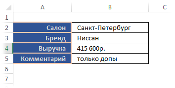
Those. in cell B2, Salon is selected from the drop-down list, and Brand is selected from B3 (you can read more about drop-down lists in the article). And depending on the choice, the amount of Revenue should be calculated and a comment should be entered. 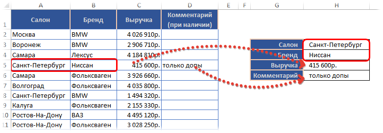
In the file attached to the article, the original table is located on the “September Report” sheet, and the second table (with selection) is on the “Selection” sheet. In fact, this is not very important; the logic of the formulas given below will simply be clearer.
The sum by two criteria can be found using the same SUMIFS:
=SUMIFS("Report September"!$C$2:$C$67;"Report September"!$A$2:$A$67; B2 ;"Report September"!$B$2:$B$67; B3)
=SUMIFS("Report September"!$C$2:$C$67,"Report September"!$A$2:$A$67,Selection!B2,"Report September"!$B$2:$B$67,Selection!B3)
You can read more about searching for amounts using two or more criteria in the article.
But with a comment it is more difficult - it contains text and SUMIFS will not find anything. And even if there are duplicates in the source data and, by definition, nothing needs to be summed, SUMIFS will not the best option- after all, it will return the sum of all cells that satisfy the conditions. And this, I repeat, is not always necessary.
Here, a function related to VLOOKUP will come to the rescue - SEARCH (MATCH):
=INDEX("Report September"!$D$2:$D$67,MATCH(B2&B3,"Report September"!$A$2:$A$67&"Report September"!$B$2:$B$67,0))
This function is . This means that it is not easy to enter it into the cells by clicking Enter, and by a combination of three keys - Ctrl+Shift+Enter. Now let's take a closer look at the principle of operation of this formula so that it can be applied to any data. In fact, the principle is not that complicated. The main emphasis is on these two “bundles”:
- B2 & B3 - here we combine the value of the selected Salon (St. Petersburg) and Brand (Nissan) into one line to get “St. PetersburgNissan”. The ampersand(&) is used to combine two values.
- “Report September”!$A$2:$A$67&“Report September”!$B$2:$B$67 - and here we consistently combine the values of two columns of the source data - Salon and Brand - into one row. Those. As a result, we will receive an array of combined values: MoscowBMW, VoronezhBMW, SamaraLexus, etc. (it is this union that requires the formula to be entered as an array formula). And already among these values we are looking for “St. PetersburgNissan”. If a match is found, MATCH will return the position of the line where it found it. And will transfer it to INDEX. And because INDEX in our case returns the value from given string of the specified array, then we get what we need.
Step by step it will look like this:
First, the searched values will be combined into one
=INDEX("Report September"!$D$2:$D$67;MATCH(B2 & B3 ;"Report September"!$A$2:$A$67&"Report September"!$B$2:$B$67;0) )
=>
=INDEX("Report September"!$D$2:$D$67;MATCH(St. Petersburg & Nissan,"Report September"!$A$2:$A$67&"Report September"!$B$2:$B$67; 0))
=>
=INDEX("Report September"!$D$2:$D$67;MATCH(St. Petersburg Nissan,"Report September"!$A$2:$A$67&"Report September"!$B$2:$B$67;0 ))
=>
then we also combine the values of all columns row by row to find the values
=INDEX("Report September"!$D$2:$D$67,MATCH(St. Petersburg Nissan,("MoscowBMW":"VoronezhBMW":"SamaraLexus":...);0))
=>
=INDEX("Report September"!$D$2:$D$67; 4
)
=>
only extras
The important thing here is to ensure that the values in the source array to be searched are concatenated in the same order as the searched values. In the attached example, if as the first argument (search_value) in MATCH we first indicated Salon(B2) and then Brand(B3), then as the second argument (lookup_array) we must specify two columns in the same order - first Salon("Report September "!$A$2:$A$67), and only then Brand("Report September"!$B$2:$B$67). If they are mixed up, this will not cause errors as such, but the values will not be found.
It is also worth considering that such a formula will take longer to calculate than the usual one, so you should not specify the columns in full (“Report September”!$A:$A), because this may entail calculating just one formula for an inordinately long time.
At the same time, it is obvious that you can view values not only from adjacent columns, but from any, and certainly they can be both the first and the last. And the returned values can also be located in any column of the table. And I also want to note that in the example only two criteria are used - in reality they can be three, five, or ten. We combine as much as necessary, indicate the required number of columns in the same way with merging and that’s it. But here you need to understand that in some cases it will be more optimal to add another column to the source data (those where we are looking) in which to record all the data, combining them. Those. again, using the file from the article as an example, you can add a formula to column E on the “September Report” sheet: = A2 & B2
and then you can search using the usual formula:
=INDEX("Report September"!$D$2:$D$67,MATCH(B2 & B3 ;"Report September"!$E$2:$E$67,0))
=INDEX("Report September"!$D$2:$D$67,MATCH(B2&B3,"Report September"!$E$2:$E$67,0))
There are no more nuances that I would like to talk about. Everything is standard, as for the usual link INDEX(SEARCH.
The example attached to the article shows an example with both the SUMIFS function and the MATCH function.
Download example:
(62.5 KiB, 522 downloads)
P.S. If someone is scared by the fact that the formula must be entered as an array formula( Ctrl+Shift+Enter), then you can modify the formula like this:
=INDEX("Report September"!$D$2:$D$67;SUMPRODUCT(MAX((B2 ="Report September"!$A$2:$A$67)*(B3 ="Report September"!$B$2:$ B$67)*(ROW($B$2:$B$67)-1))))
=INDEX("Report September"!$D$2:$D$67,SUMPRODUCT(MAX((B2="Report September"!$A$2:$A$67)*(B3="Report September"!$B$2:$ B$67)*(ROW($B$2:$B$67)-1))))
Here, instead of MATCH, the role of searching for the line number in the "Report September" array!$D$2:$D$67 is played by SUMPRODUCT. I described the very principle of operation of SUMPRODUCT in this article -. To this I can only add some clarifications (although if you want to understand the principle itself, it’s better to spend a couple of minutes on the article).
(B2 ="Report September"!$A$2:$A$67) - here the value of the selected salon is checked against the list of salons on the Report September sheet. Where the values are equal we get the value TRUE, where they differ we get FALSE.
(B3 ="Report September"!$B$2:$B$67) - here the value of the selected brand is checked against the list of brands on the Report September sheet. Where the values are equal we get the value TRUE, where they differ we get FALSE.
As a result of multiplying these two expressions, we will get an array of 1 and 0 (1 will be where the brand and salon are the same, 0 - where they differ), because TRUE for Excel is essentially =1, and FALSE =0.
Next, we multiply the resulting array of ones and zeros by the expression: LINE($B$2:$B$67) . This expression gives us an array of line numbers (2:3:4:5:6:7:8 ... etc.) because the expression takes the line number on the sheet, and we need a number in the range “Report September”!$D$2:$D$67 , then we also subtract 1 (since our range starts from the second line). With the same success, one could not subtract, but either take all ranges from the first line, or specify it like this: LINE($B$1:$B$66)
The resulting array of strings is multiplied by an array of ones and zeros for the salon and brand. As a result, we get the line number multiplied by 1 where the salon and brand are equal to the desired ones, and by zero where they differ. And as a result, an array of line numbers and zeros. And from this the maximum line number is selected.
In fact, this already solves the search problem, but if there is more than one value that matches the conditions, then this particular result may be (even most likely will be) incorrect. To avoid this, we use the MAX function so that as a result, only the maximum one is selected from all rows. Those. As a result, we will get not the first match of all possible, but the last.
I also recommend reading the article
In this lesson I will tell and show you how to use the VLOOKUP function in Excel.
IN English version this function is called VLOOKUP - stands for vertical viewing. There is also a GLOOKUP function that is focused on horizontal viewing. Basically, the VLOOKUP function is used to pull data from one table to another; it can also be used to compare columns in two different tables.
In order for us to more thoroughly understand all the features of working with a function, let's look at simple examples.
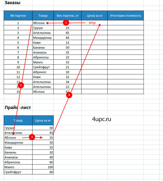
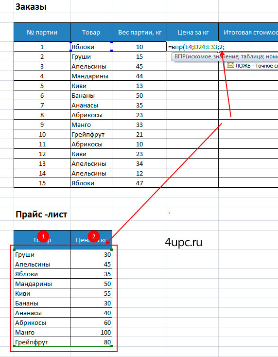
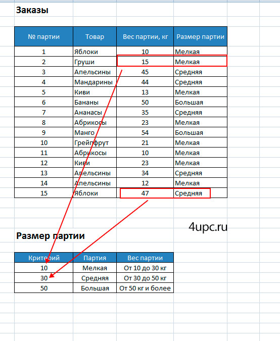
We have two tables. The first table stores data on orders for one day. It records the name of the product and the quantity of products sold by batch. The second table stores information on product prices. The task is to calculate the total revenue for each product per day.
To solve the problem, we need to pull up the prices of goods from the “Price List” table into the “Price per kg” column of the “Orders” table. Those. substitute the prices that correspond to each product from the lower table into the upper one.
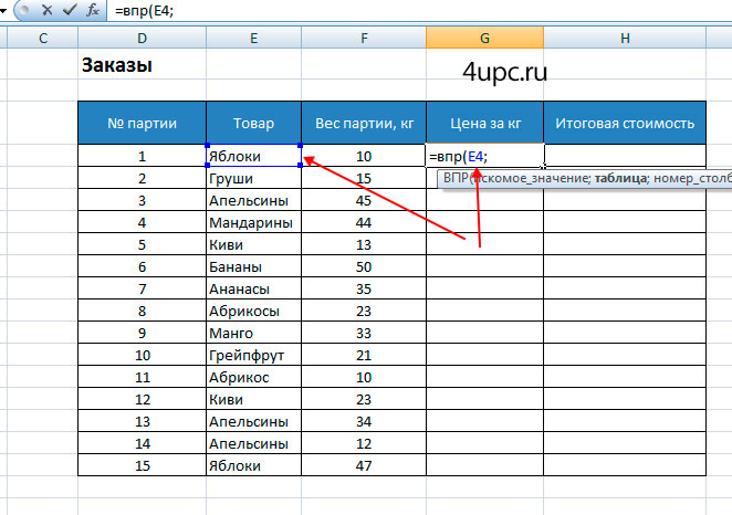
In Excel, there are several options to solve this example, one of which is to use the VLOOKUP function. We stand on the first cell where we need to substitute the data, and begin to write the function, starting as usual with the equal sign.
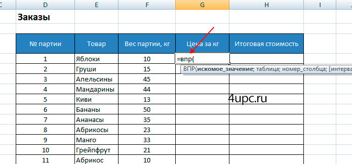
A hint should appear, according to which we will give it arguments. If we decipher the work of VLOOKUP with technical language to normal, then the VLOOKUP function will look for the product we have selected from the “Orders” table in the leftmost column of the “Price List” table and, if it finds this product, display the value of its price, which is on the same line as the found product. Briefly it looks like the screenshot below.
The VLOOKUP function has 4 arguments. The first argument that we will substitute into the formula is the same desired value, the price for which must be found in the second table “Price List”. After writing the name of the function and adding an opening parenthesis, click on the cell you are looking for and add it as an argument. In my case it is cell "E4" with the value "Apples". Next we set the separator - semicolon.
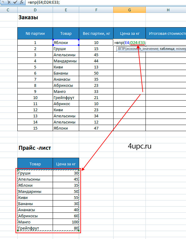
The second argument is the table in which we look for the value and from which we pull up the price. Here you just need to select the “Price List” table and it’s better that you don’t catch extra cells (header, empty cells and just unnecessary information). Don't forget to put a semicolon at the end.
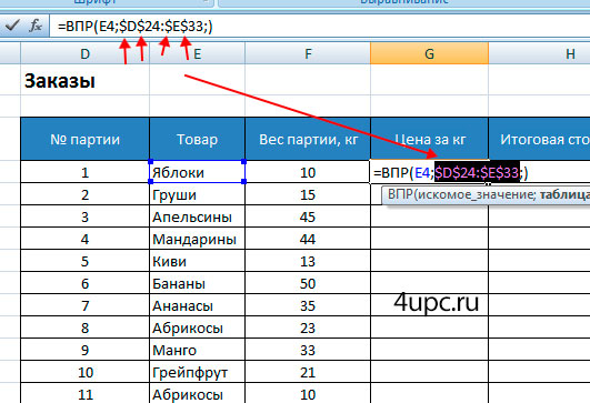
Since in our example the table in which the search is performed is located on the same sheet as the first one, when dragging the formula onto the underlying cells, the specified table will automatically slide down. To prevent this from happening, you need to select the table range inside the formula with the left mouse button and press the F4 key on the keyboard. A dollar sign will be added to the cell addresses and the table reference will turn from relative to absolute. Below we will look at cases when to create absolute links on cells will not be necessary.
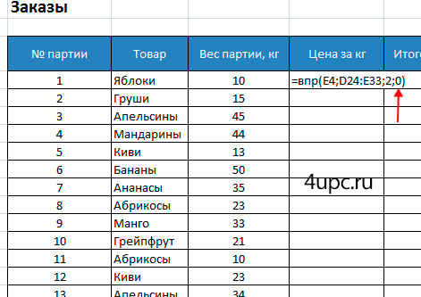
The third argument is the number of the column in the “Price List” table from which we want to pull up the value we need. In our example everything is simple. In the first column we look for the value, and from the second column we pull up the price. We put the number 2, and then a semicolon.
The last parameter is called "Interval View" - it is a Boolean argument and can only take 2 values: 0 or 1 (on/off). With this value we determine exactly the number 0, or approximately the number 1, we are looking for the name in the price list. In the case of text names, it is better to use an exact search (number 0), because the approximate search works more or less accurately in the case of cells with numbers. Enter the interval view as 0 and close the bracket. After that, click Enter key for the formula to work. As a result, we will get a cell with a price pulled from the price list table.

In the “Total cost” column we write a simple formula for multiplying the weight of the batch by the price per kg.

Select both cells and, holding left key mouse on the lower right corner of the selection, drag the formulas down to all the remaining cells.

As a result, we get the price and final cost of each batch. At further use The obtained data should not be forgotten that they are the result of the formula, and not ready-made values. In order to be able to work with them in the future, you need to copy the cells with the resulting data and paste them back into their place via paste special as normal values.

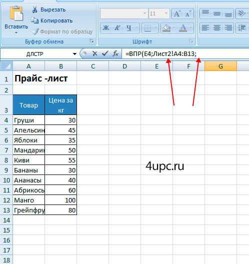
We have discussed with you one of the cases when there is a need to pull up data from a table that is located on the same sheet. Of course, you can use tables that are on different sheets and even when they are open in different documents. In this case, the second argument to the function will look a little different. In the case of another sheet or document, it is not at all necessary to specify absolute links, and it is better to add the third and fourth arguments in the function input field, without returning back to the sheet where you started typing it.
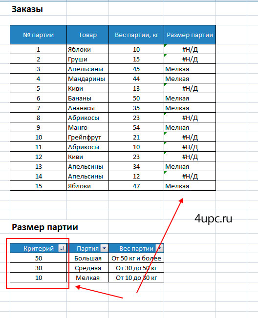
Another useful one using VPR is its use to compare two tables in order to find matches or differences. For example, if you remove several rows from one of the tables, then there will no longer be a complete match in the data and the inscription #N/A will appear in some cells. This inscription indicates that the values from the table with orders were not found in the price list table, which accordingly leads to an error.

Now let's look at a case where there is a need to use interval viewing, not exact, with the number 0, but approximate, with the number 1. This method is rarely used, but nevertheless there are tasks in which you may need it.
Let's return to our table with orders and try to determine the size of the batch by its weight. We will have a table with orders and a table with batch parameters.
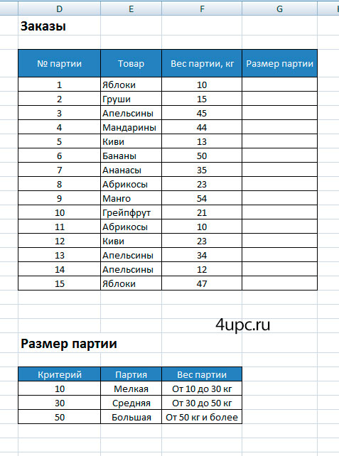
Additionally, we have a “from and to” criterion, which indicates the size of the batch. In the example, we will start from its weight. For example, if Excel shows the weight of a batch of 15 kg, then it will understand that this is a small batch.
Let's figure out how it works. We begin to write the VLOOKUP function, but at the end of the formula we put not 0, but 1. In the argument where we need to specify a table with cells, we will not specify a column with the “From and to” parameter, since Excel will not understand such an entry. Instead, we introduce a criterion field, which will determine the beginning and end of the weight range. At the end, press the Enter key and drag across all cells.


There are some features of the work that need to be explained so that it is clear what happened here. We see that at a certain weight, the function pulled a certain batch from the second table. To understand the logic more precisely, let's look at the weight, for example, 15 kg. In the table with batch sizes, there is no such criterion. But when we set the interval lookup to 1, the function will pull out the value which is the nearest smaller one. If the batch weight is 15 kg, VLOOKUP will pull out a value with criterion 10 from the table. If the batch weight is 47 kg, then the function will pull out a value with criterion 30, which will be the closest and smaller.
When working with a function in this mode, there is a very important point, which you should consider. The criteria must be sorted in ascending order - from smallest to largest. If the criteria are sorted in reverse order, then the function will not work.
That's all for the function. I hope that with these examples you will learn how to work with the VLOOKUP function. If you have any difficulties, be sure to ask them in the comments below.
New TOP project from a reliable admin, REGISTER!
Stay up to date with site updates, be sure to subscribe to the channel Youtube and group
The VLOOKUP function in the table will help you find the value in the table. Excel examples which are described below in the article.
While working with the program, users often need to quick search information in one table and transferring it to another sheet object.
Understanding the principle VPR work will significantly simplify your work in Excel and will help you complete tasks faster.
VLOOKUP (Vertical Lookup) is another function name that can be found in the English version of the spreadsheet processor. The abbreviation VPR itself means “vertical viewing”. Analysis of data and its search in the table is carried out using gradual enumeration of elements from row to row in each column.
Also, Excel has the opposite function called HLOOKUP or HLOOKUP - horizontal viewing. The only difference in the operation of the options is that GLOOK performs a search in the table by enumerating columns, not rows. More often, users prefer the VLOOKUP function, because most tables have more rows than columns.
What does VLOOKUP syntax look like?
The syntax of a function in Excel is a set of parameters with which it can be called and set. The recording is similar to the recording method mathematical functions. Look correct view options can be opened by opening table processor :
- Use an already created document, or open a new blank sheet;
- Click on the “Formulas” button, as shown in the figure below;
- In the search bar, type “VLOOKUP” or “VLOOKUP” depending on the program language;
- Set up a category "Full list";
- Click on "Find".
Fig. 2 – search for formulas in Excel
As a result of searching for a formula, you will see it in the list. By clicking on an element, its formula will be displayed at the bottom of the screen. The name of the function is indicated outside the brackets, and its parameters are inside the brackets. Inside the formula each separate parameter written in corner<>staples. General form The description for the VLOOKUP looks like this:
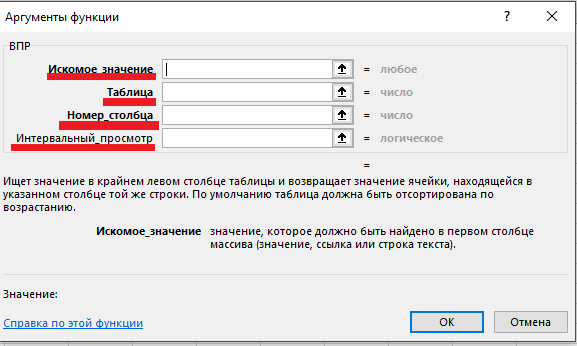
Fig.3 – list of parameters
Let's take a closer look at each of the values, which are described in brackets:
- <ЧТО>- the first element. Instead, you need to enter exactly the value that you want to find in the table. You can also enter the cell address in the table;
- <НОМЕР_СТОЛБЦА>- here you need to print the number of the column within which the data will be sorted.
- <ГДЕ>- here the user determines the number of cells, specifying their dimension in the form two-dimensional array data. The first column is the “WHAT” element;
- <ОТСОРТИРОВАНО>- this element of the VLOOKUP function is responsible for sorting the first column in ascending order (the first column is for “WHERE”). As a result of successful sorting, the value becomes true (one). If any inaccuracies or errors occur while entering parameters, a false sorting value (zero) appears. It is worth noting that during the VLOOKUP task<ОТСОРТИРОВАНО>can be omitted, in which case its default value is accepted as true.
How VLOOKUP works. Useful example
To better understand the principle of operation of VLOOKUP, let's move on to consider specific examples. Let's take the simplest table with two columns. Let it indicate the code and name of the product.
After filling out the table, click on an empty cell and let's write the formula into it and the result of the VPR. Click on the Formulas tab and select VLOOKUP. Then enter everything required parameters into the window shown in Figure 3. Confirm the action. The cell will display the result of the command.
![]()
Fig. 4 – example of searching in a simple table
In the picture above, the colored cells indicate the value for the product. If you do not enter a value to sort, the function automatically treats it as one. Next, the program “thinks” that the elements of the first column of your table are in ascending order from top to bottom. Thanks to this, the search procedure will be stopped only when a line with a value is reached, the number of which is already higher than the searched object.
Let's look at another example of using a function that is often encountered during real work with price lists and product name sheets. In the case where the user types that the last element in brackets equal to zero, Excel works like this:: The option checks the very first column in the given array range. The search will be stopped automatically as soon as a match is found between the “WHAT” parameter and the product name.
If the table does not have the identifier you entered for the product name, the VLOOKUP search will return N/A, which means there is no item for the given number.
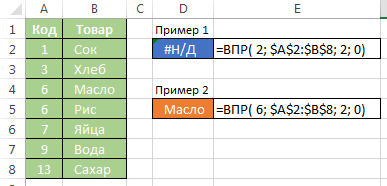
Fig.5 – second example for VLOOKUP
When to use VLOOKUP?
Two options for using VLOOKUP are described above.
First variation VLOOKUP suitable for the following cases:
- When it is necessary to divide the values of a table processor object by its ranges;
- For those tables in which the WHERE parameter can contain several identical values. In this case, the formula will return only the one that is in the last line of the array;
- When to look for values that Furthermore, which may be contained in the first column. So you will find last line tables almost instantly.
First spelling VLOOKUP cannot find an element unless a value less than or equal to the search value was found . Only "N/A" will be returned in the result cell.
Second option for VPR (specifying "0" for sorting) is used for large tables, in which they meet same names for several cells. VLOOKUP makes it easy to manipulate data because it returns the first row found.
IN real life This option is used when you need to search within a given range - it does not have to correspond to the entire table size. In worksheet objects that contain different types of values, VLOOKUP helps you find text strings.
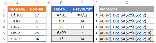
Fig. 6 – example of searching for a text value
VLOOKUP is useful when you need to delete a lot extra spaces. The function quickly finds all names with spaces, and you can quickly delete them. Example:

Fig.7 – VLOOKUP when removing spaces
PerformanceVLOOKUP
Most users prefer not to enter the parameter<СОРТИРОВКА> while working with the function. Of course, it’s easier to enter zero, but ignoring the operator slows down the search. When working with large amounts of data, Excel can be too slow. On older devices, the table processor sometimes even freezes due to the VLOOKUP search being too slow.
If there are several thousand formulas on one sheet of your document, it is better to take care of sorting the first column. This allows you to increase overall performance search by as much as 400%-500%.
Such a difference in execution speed different types VLOOKUP is that any computer program It is much easier to work with already sorted data by performing a binary search. The first type of function uses binary search, but the second does not, because optimization of this method of specifying a function is still missing.


