What are the types of data structures? Data structures: general concept, implementation. The simplest data structures: queue, stack. Using a stack and reverse Polish notation
The concept of data structure is so fundamental that it is difficult to find a simple definition for it. The task becomes easier if we try to formulate this concept in relation to data types and variables. As you know, a program is a unity of an algorithm (procedures, functions) and the data they process. Data, in turn, are defined by basic and derived data types - “ideal” representations of fixed-dimensional variables with sets of known operations on them and their components. Variables are named areas of memory into which constructed data types are "mapped".
In a program, it is always possible to distinguish groups of indirectly related (by using data in the same procedures and functions) and directly related (by the presence of relationships through pointers) variables. To a first approximation, they can be considered data structures.
There are SIMPLE (basic, primitive) data structures (types) and INTEGRATED (structured, composite, complex). Simple data structures are those that cannot be broken down into components larger than bits. From the point of view of physical structure, the important fact is that in a given machine architecture, in a given programming system, we can always tell in advance what the size of a given simple type will be and what the structure of its placement in memory will be. From a logical point of view, simple data are indivisible units. Integrated are those data structures whose components are other data structures - simple or, in turn, integrated. Integrated data structures are constructed by the programmer using the data integration tools provided by programming languages.
Depending on the absence or presence of explicitly defined connections between data elements, one should distinguish between DISCONNECTED structures (vectors, arrays, strings, stacks, queues) and LINKED structures (linked lists).
A very important feature of a data structure is its variability - a change in the number of elements and (or) connections between the elements of the structure. The definition of structure variability does not reflect the fact that the values of data elements change, since in this case all data structures would have the property of variability. Based on variability, structures are distinguished: STATIC, SEMI-STATIC, DYNAMIC. The classification of data structures based on variability is shown in Fig. 1.1. Basic data structures, static, semi-static and dynamic, are characteristic of RAM and are often called operational structures. The file structures correspond to the data structures for external memory.
Rice. 1.1. Classification of data structures
An important feature of a data structure is the ordering nature of its elements. Based on this feature, structures can be divided into LINEAR AND NON-LINEAR structures.
Depending on the nature of the relative arrangement of elements in memory, linear structures can be divided into structures with CONSEQUENTIAL distribution of elements in memory (vectors, strings, arrays, stacks, queues) and structures with ARBITRARY CONNECTED distribution of elements in memory (simply linked, doubly linked lists). An example of nonlinear structures is multi-linked lists, trees, graphs.
In programming languages, the concept of “data structures” is closely related to the concept of “data types”. Any data, i.e. constants, variables, function values or expressions are characterized by their types.
Information for each type clearly identifies:
· 1) data storage structure of the specified type, i.e. allocating memory and representing data in it, on the one hand, and interpreting the binary representation, on the other;
· 2) the set of permissible values that this or that object of the described type can have;
· 3) a set of valid operations that are applicable to an object of the described type.
DATA STRUCTURE is a set of physically (data types) and logically (algorithm, functions) interrelated variables and their values.
Note that the concept of a data structure relates not only to the variables that make it up, but also to algorithms (functions) that not only logically connect the variables with each other, but also determine the internal values that should also be characteristic of this data structure. For example, a sequence of positive values placed in an array and having a variable dimension (data structure) may have a null delimiter. All operations for generating and checking this limiter are implemented by functions. Thus, we can say that a significant part of the data structure is “hard-wired” in the algorithms for its processing.
The method of defining variables through data types known to us is characterized by the fact that, firstly, the number of variables in the program is fixed, and secondly, their dimension cannot be changed while the program is running. If the relationships between these variables are more or less constant, then such data structures can be called static.
STATIC DATA STRUCTURE - a set of a fixed number of variables of constant dimension with the unchanged nature of the connections between them
Conversely, if one of the parameters of the data structure—the number of variables, their dimension, or the relationships between them—changes while the program is running, then such data structures are called dynamic.
DYNAMIC DATA STRUCTURE - a set of variables, the number, dimension or nature of the relationships between which changes during program operation.
Dynamic data structures are based on two programming language elements:
· dynamic variables, the number of which can change and is ultimately determined by the program itself. In addition, the ability to create dynamic arrays allows us to talk about data of variable dimensions;
· pointers that provide a direct relationship between data and the ability to change these connections.
Thus, the following definition is close to the truth: dynamic data structures are dynamic variables and arrays linked by pointers.
Speaking about data structures, we must not forget that ordinary variables are located in RAM (internal memory of the computer). Therefore, data structures usually also have something to do with memory. However, there is also external memory, which in the language is accessible indirectly through operators (Pascal) or functions (C) that work with files. In binary random access mode, any file is analogous to an unlimited directly addressable memory region, that is, from the program's point of view, it looks the same as regular memory. Naturally, the program can copy variables from memory to an arbitrary location in the file and back, and therefore organize any (including dynamic) data structures in the file.
A data structure is an executor who organizes work with data, including its storage, addition and deletion, modification, search, etc. The data structure maintains a certain order of access to it. A data structure can be thought of as a kind of warehouse or library. When describing a data structure, you need to list the set of actions that are possible for it and clearly describe the result of each action. We will call such actions prescriptions. From a programming point of view, a system of data structure prescriptions corresponds to a set of functions that operate on common variables.
Data structures are most conveniently implemented in object-oriented languages. In them, the data structure corresponds to a class, the data itself is stored in class member variables (or data is accessed through member variables), and a set of class methods corresponds to a system of prescriptions. As a rule, in object-oriented languages, data structures are implemented in the form of a library of standard classes: these are the so-called container classes of the C++ language, included in the standard STL class library, or classes that implement various data structures from the Java Developer Kit library of the Java language.
However, data structures can be implemented just as successfully in traditional programming languages such as Fortran or C. In this case, you should adhere to the object-oriented programming style: clearly identify a set of functions that work with the data structure, and limit access to data only to this set of functions. The data itself is implemented as static (not global) variables. When programming in the C language, the data structure corresponds to two files with source texts:
1. header, or h-file, which describes the interface of the data structure, i.e. a set of function prototypes corresponding to a system of data structure prescriptions;
2. implementation file, or C-file, which defines static variables that store and access data, and also implements functions that correspond to the system of data structure requirements
The data structure is usually implemented based on a simpler base structure already implemented, or based on an array and a set of simple variables. A clear distinction should be made between describing a data structure from a logical point of view and describing its implementation. There can be many different implementations, but from a logical point of view (i.e., from the point of view of an external user), they are all equivalent and differ, perhaps, only in the speed of executing instructions.
- Translation
Of course, you can be a successful programmer without sacred knowledge of data structures, but they are absolutely indispensable in some applications. For example, when you need to calculate the shortest path between two points on a map, or find a name in a phone book containing, say, a million entries. Not to mention, data structures are used all the time in sports programming. Let's look at some of them in more detail.
Queue
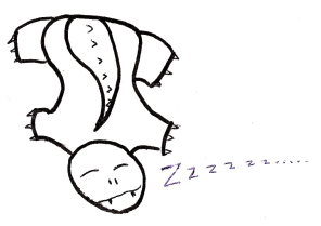
So say hello to Loopy!
Loopy loves playing hockey with his family. And by “game,” I mean:

When the turtles fly into the gate, they are thrown to the top of the stack. Note that the first turtle added to the pile is the first to leave it. It is called Queue. Just like in the queues that we see in everyday life, the first element added to the list is the first to leave it. This structure is also called FIFO(First In First Out).
What about insert and delete operations?
Q = def insert(elem): q.append(elem) #add an element to the end of the queue print q def delete(): q.pop(0) #remove the zero element from the queue print q
Stack
After such a fun game of hockey, Loopy makes pancakes for everyone. She puts them in one pile.
When all the pancakes are ready, Loopy serves them to the whole family, one by one.

Note that the first pancake she makes will be served last. It is called Stack. The last element added to the list will be the first to leave it. This data structure is also called LIFO(Last In First Out).
Adding and removing elements?
S = def push(elem): #Add an element to the stack - Push s.append(elem) print s def customPop(): #Remove an element from the stack - Pop s.pop(len(s)-1) print s
Heap
Have you ever seen a density tower?
All elements from top to bottom are located in their places, according to their density. What happens if you throw a new object inside?

It will take up space depending on its density.
This is roughly how it works Heap.

A heap is a binary tree. This means that each parent element has two children. And although we call this data structure a heap, it is expressed through a regular array.
Also the heap always has a height of logn, where n is the number of elements
The figure shows a max-heap based on the following rule: children less parental. There are also min-heap heaps, where children are always more parental.
A few simple functions for working with heaps:
Global heap global currSize def parent(i): #Get the index of the parent for the i-th element return i/2 def left(i): #Get the left child of the i-th element return 2*i def right(i): #Get right child of i-th return (2*i + 1)
Adding an element to an existing heap
To begin with, we add an element to the very bottom of the heap, i.e. to the end of the array. We then swap it with its parent element until it fits into place.

Algorithm:
- Add an element to the very bottom of the heap.
- Compare the added element with the parent; If the order is correct, we stop.
- If not, swap the elements and return to the previous point.
Def swap(a, b): #swap the element with index a for the element with index b temp = heap[a] heap[a] = heap[b] heap[b] = temp def insert(elem): global currSize index = len(heap) heap.append(elem) currSize += 1 par = parent(index) flag = 0 while flag != 1: if index == 1: #We reached the root element flag = 1 elif heap > elem: #If the index of the root element is greater than the index of our element - our element is in its place flag = 1 else: #Swap the parent element with our swap(par, index) index = par par = parent(index) print heap
The maximum number of passes of the while loop is equal to the height of the tree, or logn, hence the complexity of the algorithm is O(logn).
Retrieving the maximum heap element
The first element in the heap is always the maximum, so we will simply remove it (after remembering it first), and replace it with the lowest one. We will then put the heap in the correct order using the function:
MaxHeapify().

Algorithm:
- Replace the root element with the bottom element.
- Compare the new root element with its children. If they are in the right order, stop.
- If not, replace the root element with one of the children (smaller for min-heap, larger for max-heap), and repeat step 2.
Def extractMax(): global currSize if currSize != 0: maxElem = heap heap = heap #Replace the root element with the last one heap.pop(currSize) #Remove the last element currSize -= 1 #Reduce the heap size maxHeapify(1) return maxElem def maxHeapify(index): global currSize lar = index l = left(index) r = right(index) #Calculate which child element is larger; if it is larger than the parent one, swap places if l<= currSize and heap[l] >heap: lar = l if r<= currSize and heap[r] >heap: lar = r if lar != index: swap(index, lar) maxHeapify(lar)
Again, the maximum number of calls to the maxHeapify function is equal to the height of the tree, or logn, which means the complexity of the algorithm is O(logn).
We make a heap from any random array
Okay, there are two ways to do this. The first is to insert each element into the heap one by one. It's simple, but completely ineffective. The complexity of the algorithm in this case will be O(nlogn), because the O(logn) function will be executed n times.
A more efficient way is to use the maxHeapify function for ‘ sub-heaps', from (currSize/2) to the first element.
The complexity will be O(n), and the proof of this statement, unfortunately, is beyond the scope of this article. Just understand that elements in the currSize/2 to currSize portion of the heap have no children, and most of the 'sub-heaps' created this way will be less than logn in height.
Def buildHeap(): global currSize for i in range(currSize/2, 0, -1): #the third argument in range() is the search step, in this case it determines the direction. print heap maxHeapify(i) currSize = len(heap)-1 
Really, why is all this?
Heaps are needed to implement a special type of sorting called, oddly enough, “ heap sort" Unlike the less efficient “insertion sort” and “bubble sort,” with their terrible O(n2) complexity, “heap sort” has O(nlogn) complexity.
The implementation is indecently simple. Just keep popping the maximum (root) element from the heap sequentially, and writing it to the array until the heap is empty.
Def heapSort(): for i in range(1, len(heap)): print heap heap.insert(len(heap)-i, extractMax()) #insert the maximum element at the end of the array currSize = len(heap)-1
To summarize all of the above, I wrote a few lines of code containing functions for working with the heap, and for OOP fans, I formatted everything as a class.
Easy, isn't it? Here comes the celebrating Loopy!

Hash
Loopy wants to teach her kids to recognize shapes and colors. To do this, she brought home a huge number of colorful figures.
After a while the turtles became completely confused

So she pulled out another toy to make the process a little easier.

It became much easier, because the turtles already knew that the figures were sorted by shape. What if we labeled every pillar?

The turtles now need to check a pillar with a certain number, and choose the right one from a much smaller number of figures. What if we also have a separate pillar for each combination of shape and color?
Let's say the column number is calculated as follows:
Full name summer tre square
f+i+o+t+r+e = 22+10+16+20+18+6 = Column 92
Kra sleepy straight triangle
k+p+a+p+p+i = 12+18+1+17+18+33 = Column 99
We know that 6*33 = 198 possible combinations, which means we need 198 pillars.
Let's call this formula for calculating the column number - Hash function.
Code:
def hashFunc(piece): words = piece.split(" ") #split the string into words color = words shape = words poleNum = 0 for i in range(0, 3): poleNum += ord(colour[i]) - 96 poleNum += ord(shape[i]) - 96 return poleNum
(with Cyrillic it’s a little more complicated, but I left it that way for simplicity. - approx.)
Now, if we were to find out where the pink square is stored, we can calculate:
hashFunc("pink square")

This is an example of a hash table where the location of the elements is determined by a hash function.
With this approach, the time spent searching for any element does not depend on the number of elements, i.e. O(1). In other words, the search time in a hash table is a constant value.
Okay, but let's say we are looking for “ car amel straight triangle” (if, of course, the color “caramel” exists).
HashFunc("caramel rectangle")
will return us 99, which is the same number for the red rectangle. It is called " Collision" To resolve a collision we use “ Chain method”, implying that each column stores a list in which we look for the record we need.
So we just put the candy rectangle on the red one, and pick one when the hash function points to that pillar.
The key to a good hash table is choosing an appropriate hash function. This is hands down the most important thing in creating a hash table, and people spend a huge amount of time developing quality hash functions.
In good tables, no position contains more than 2-3 elements; otherwise, hashing does not work well, and you need to change the hash function.

Once again, search independent of the number of elements! We can use hash tables for anything that is gigantic in size.
Hash tables are also used to find strings and substrings in large chunks of text using the algorithm Rabin-Karp or algorithm Knuth-Morris-Pratt, which is useful, for example, for identifying plagiarism in scientific papers.
I think we can finish here. In the future I plan to look at more complex data structures, e.g. Fibonacci pile And Segment tree. I hope you found this informal guide interesting and useful.
Translated for Habr locked on
Exam Computer Science
Information as a resource. Methods of storing and processing information.
Information from Lat. "Information" means clarification, awareness, presentation.
In a broad sense information – This is a general scientific concept that includes the exchange of information between people, the exchange of signals between living and inanimate nature, people and devices.
Information – This is information about objects and phenomena of the environment, their parameters, properties and condition, which reduce the degree of uncertainty and incomplete knowledge about them.
Computer science examines information as conceptually interconnected information, data, concepts that change our ideas about a phenomenon or object in the surrounding world.
Informational resources - these are individual documents and separate arrays of documents, documents and arrays of documents in information systems (libraries, archives, funds, banks).
In order for information to be used, and repeatedly, it must be stored.
Data storage - it is a way of disseminating information in space and time. The method of storing information depends on its medium (book - library, painting - museum, photograph - album). A computer is designed for compact storage of information with the ability to quickly access it.
Data processing is the transformation of information from one type to another.
Information processing - the very process of transition from initial data to the result is the processing process. The object or subject carrying out the processing is the performer of the processing.
1st type of processing: processing associated with obtaining new information, new knowledge content.
2nd type of processing: processing associated with a change in form, but not changing the content (for example,
translation of text from one language to another).
An important type of processing is coding– transformation of information into symbolic form,
convenient for its storage, transmission, processing. Another type of information processing is data structuring (entering a certain order into the information storage, classification, cataloging of data).
Another type of information processing is searching in some information storage for the necessary data that satisfies certain search conditions (query).
The concept of structured data. Definition and purpose of a database.
When creating a database, the user strives to organize information according to various characteristics and quickly retrieve a sample with an arbitrary combination of characteristics. This can only be done if the data is structured.
Structuring - it is the introduction of conventions on how data should be presented.
Structured data - this is ordered data.
Unstructured data – this is data recorded, for example, in a text file: Personal file No. 1 Oleg Ivanovich Sidorov, date of birth. 11/14/92, Personal file No. 2 Petrova Anna Viktorovna, date of birth. 03/15/91.
To automate the search and systematize this data, it is necessary to develop certain agreements on how to provide data, i.e. date of birth must be written down the same way for each student, it must have the same length and definition. place among the rest of the information. The same remarks apply to the rest of the data (personal file number, F., I., O.) After carrying out a simple structuring of the information, it will look like this:
Example of structured data: No. Full name Date of birth
1 Sidorov Oleg Ivanovich 11/14/92
Structured Data Elements:
1) A – field (column) – is an elementary indivisible unit of information organization
2) B – record (line) is a collection of logically related fields
3) B – table (file) is a collection of instances of records of the same structure.
Database - This is a set of interconnected structured data organized on computer media, containing information about various entities of a certain subject area (objects, processes, events, phenomena).
In the broad sense of the word, a database is a collection of information about specific objects of the real world in any subject area.
Under subject area is understood as a part of the real world that is subject to study for the organization of management, automation, for example, an enterprise, a university, etc.
Database purpose:
1)Data redundancy control. As already mentioned, traditional file systems waste external memory by storing the same data in multiple files. In contrast, using a database attempts to eliminate data redundancy by integrating files to avoid storing multiple copies of the same piece of information.
2) Data consistency. Eliminating or controlling data redundancy reduces the risk of inconsistent conditions. If a data element is stored in the database in only one instance, then changing its value will require only one update operation, and the new value will be immediately available to all users of the database. And if this data element, with the knowledge of the system, is stored in the database in several copies, then such a system will be able to ensure that the copies do not contradict each other.
3)Data sharing. Files are usually owned by individuals or entire departments who use them in their work. At the same time, the database belongs to the entire organization and can be shared by all registered users. With this organization of work, more users can work with a larger amount of data. Moreover, you can create new applications based on information that already exists in the database and add only the data that is not currently stored in it, rather than redefining the requirements for all the data needed by the new application.
4) Maintaining data integrity. Database integrity means the correctness and consistency of the data stored in it. Integrity is usually described using constraints, i.e. rules for maintaining consistency that should not be violated in the database. Constraints can be applied to data elements within a single record or to relationships between records. For example, an integrity constraint may state that an employee’s salary should not exceed 40,000 rubles per year, or that in an employee’s data record, the number of the department in which he works must correspond to an actual department of the company.
5) Increased security. Database security is about protecting the database from unauthorized access by users. Without appropriate security measures in place, integrated data becomes more vulnerable than data in the file system. However, integration allows you to determine the required database security system, and the DBMS to implement it. The security system can be expressed in the form of login names and passwords to identify users who are registered in this database. Access to data by a registered user can be limited to only certain operations (extract, insert, update and delete).


