Regression in Excel explained. Correlation analysis in Excel. Activate the Analysis Package

In my opinion, as a student, econometrics is one of the most applied sciences that I was able to get acquainted with within the walls of my university. With its help, it is indeed possible to solve applied problems on an enterprise scale. How effective these decisions will be is the third question. The point is that most of the knowledge will remain theory, but econometrics and regression analysis Still worth studying with special attention.

What does regression explain?

Before we begin to consider the functions of MS Excel that allow us to solve these problems, I would like to explain to you in detail what regression analysis, in essence, involves. This will make it easier for you to pass the exam, and most importantly, it will be more interesting to study the subject.

Hopefully you are familiar with the concept of a function from mathematics. A function is the relationship between two variables. When one variable changes, something happens to another. We change X, and Y changes accordingly. Functions describe various laws. Knowing the function, we can substitute arbitrary values of X and see how Y changes.

It has great importance, since regression is an attempt to explain, at first glance, unsystematic and chaotic processes using a certain function. For example, it is possible to identify the relationship between the dollar exchange rate and unemployment in Russia.

If this pattern can be discovered, then using the function we obtained during the calculations, we will be able to make a forecast of what the unemployment rate will be at the Nth dollar exchange rate against the ruble.
This relationship will be called correlation. Regression analysis involves calculating a correlation coefficient that will explain the close relationship between the variables we are considering (the dollar exchange rate and the number of jobs).

This coefficient can be positive or negative. Its values range from -1 to 1. Accordingly, we can observe a high negative or positive correlation. If it is positive, then the increase in the dollar exchange rate will be followed by the creation of new jobs. If it is negative, it means that an increase in the exchange rate will be followed by a decrease in jobs.

There are several types of regression. It can be linear, parabolic, power, exponential, etc. We choose a model depending on which regression will correspond specifically to our case, which model will be as close as possible to our correlation. Let's look at this using an example problem and solve it in MS Excel.

Linear Regression in MS Excel

To solve linear regression problems, you will need the Data Analysis functionality. It may not be enabled for you, so you need to activate it.

Click on the “File” button;
Select the “Options” item;
Click on the penultimate tab “Add-ons” on the left side;

Below we will see the inscription “Management” and the “Go” button. Click on it;
Check the box for “Analysis package”;
Click “ok”.

Sample task

The batch analysis function is activated. Let's solve the following problem. We have a sample of data for several years on the number of emergency situations on the territory of the enterprise and the number of employed workers. We need to identify the relationship between these two variables. There is an explanatory variable X - this is the number of workers and an explanatory variable - Y - this is the number of emergency incidents. Let's distribute the source data into two columns.

Let's go to the “data” tab and select “Data analysis”

In the list that appears, select “Regression”. In the input intervals Y and X we select the appropriate values.

Click "Ok". The analysis is completed, and we will see the results in a new sheet.

The most significant values for us are marked in the figure below.

Multiple R is the coefficient of determination. It has a complex calculation formula and shows how much you can trust our correlation coefficient. Accordingly, the higher this value, the more trust, the more successful our model as a whole.

Y-Intercept and X1-Intercept are our regression coefficients. As already mentioned, regression is a function, and it has certain coefficients. Thus, our function will look like: Y = 0.64*X-2.84.

What does this give us? This gives us the opportunity to make a forecast. Let's say we want to hire 25 workers for an enterprise and we need to roughly imagine what the number of emergency incidents will be. We substitute it into our function given value and we get the result Y = 0.64 * 25 – 2.84. We will have approximately 13 emergencies.

Let's see how it works. Take a look at the picture below. The actual values for the involved employees are substituted into the function we received. See how close the values are to real players.

You can also build a correlation field by selecting the area of the Y's and X's, clicking on the "insert" tab and selecting the scatter plot.

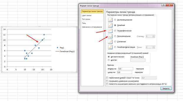
The dots are scattered, but generally move upward, as if there is a straight line in the middle. And you can also add this line by going to the “Layout” tab in MS Excel and selecting “Trend Line”

Double-click on the line that appears and you will see what was mentioned earlier. You can change the regression type depending on what your correlation field looks like.

You may feel that the points draw a parabola rather than a straight line and that it would be better for you to choose a different type of regression.

Conclusion

Hopefully, this article has given you a greater understanding of what regression analysis is and why it is needed. All this is of great practical importance.

This is the most common way to show the dependence of some variable on others, for example, how does GDP level from the size foreign investment or from National Bank lending rate or from prices for key energy resources.

Modeling allows you to show the magnitude of this dependence (coefficients), thanks to which you can make a direct forecast and carry out some kind of planning based on these forecasts. Also, based on regression analysis, it is possible to make management decisions aimed at stimulating priority causes affecting final result, the model itself will help highlight these priority factors.

General view of the linear regression model:

Y=a 0 +a 1 x 1 +...+a k x k

Where a - regression parameters (coefficients), x - influencing factors, k - number of model factors.

Initial data

Among the initial data, we need a certain set of data that would represent several consecutive or interconnected values of the final parameter Y (for example, GDP) and the same number of values of the indicators whose influence we are studying (for example, foreign investment).

The figure above shows a table with these same initial data, Y is an indicator of the economically active population, and the number of enterprises, the amount of investment in capital and household income are influencing factors, that is, X's.

Based on the figure, one can also make an erroneous conclusion that modeling can only be about time series, that is, moment series recorded sequentially in time, but this is not the case; with the same success, one can model in terms of structure, for example, the values indicated in the table can be broken down not by year, but by region.

To build adequate linear models It is desirable that the source data does not have strong drops or collapses; in such cases, it is advisable to carry out smoothing, but we will talk about smoothing next time.

Analysis package

The parameters of a linear regression model can also be calculated manually using the Ordinary Least Squares Method (OLS), but this is quite time-consuming. This can be calculated a little faster using the same method by using formulas in Excel, where the program itself will do the calculations, but you will still have to enter the formulas manually.

Excel has an add-in Analysis package which is pretty powerful tool to help the analyst. This toolkit, among other things, can calculate regression parameters using the same least squares method, in just a few clicks. In fact, how to use this tool will be discussed further.

Activate the Analysis Package

By default, this add-on is disabled and you won’t find it in the tab menu, so we’ll take a step-by-step look at how to activate it.

In Excel, at the top left, activate the tab File, in the menu that opens, look for the item Options and click on it.

In the window that opens, on the left, look for the item Add-ons and activate it, in this tab at the bottom there will be a drop-down control list, where by default it will be written Excel add-ins , there will be a button to the right of the drop-down list Go, you need to click on it.

A pop-up window will prompt you to select available add-ons; in it you need to check the box Analysis package and at the same time, just in case, Finding a solution(also a useful thing), and then confirm your choice by clicking on the button OK.

Instructions for finding linear regression parameters using the Analysis Package

After activating the Analysis Pack add-on, it will always be available in the main menu tab Data under the link Data analysis

In the active tool window Data Analysis from the list of possibilities we search and select Regression

Next, a window will open for setting up and selecting source data for calculating the parameters of the regression model. Here you need to indicate the intervals of the initial data, namely the parameter being described (Y) and the factors influencing it (X), as shown in the figure below; the remaining parameters, in principle, are optional to configure.

After you have selected the source data and clicked the OK button, Excel produces calculations on a new sheet of the active workbook (unless it was set otherwise in the settings), these calculations look like this:

Key cells filled yellow These are the ones you need to pay attention to first of all, the other parameters are also important, but their detailed analysis Perhaps requires a separate post.

So, 0,865 - This R 2- coefficient of determination, showing that 86.5% of the calculated parameters of the model, that is, the model itself, explain the dependence and changes in the parameter being studied - Y from the studied factors - X's. If exaggerated, then this is an indicator of the quality of the model and the higher it is, the better. It is clear that it cannot be more than 1 and is considered good when R 2 is above 0.8, and if it is less than 0.5, then the reasonableness of such a model can be safely questioned.

Now let's move on to model coefficients:
2079,85 - This a 0- a coefficient that shows what Y will be if all factors used in the model are equal to 0, it is understood that this is a dependence on other factors not described in the model;
-0,0056 - a 1- a coefficient that shows the weight of the influence of factor x 1 on Y, that is, the number of enterprises within a given model affects the indicator of the economically active population with a weight of only -0.0056 (a rather small degree of influence). The minus sign shows that this influence is negative, that is, the more enterprises, the less economically active population, no matter how paradoxical this may be in meaning;
-0,0026 - a 2- coefficient of influence of the volume of investments in capital on the size of the economically active population; according to the model, this influence is also negative;
0,0028 - a 3- coefficient of influence of population income on the size of the economically active population, here the influence is positive, that is, according to the model, an increase in income will contribute to an increase in the size of the economically active population.

Let's collect the calculated coefficients into the model:

Y = 2079.85 - 0.0056x 1 - 0.0026x 2 + 0.0028x 3

Actually, this is linear regression model, which for the source data used in the example looks exactly like this.

Model estimates and forecast

As we have already discussed above, the model is built not only to show the magnitude of the dependence of the parameter being studied on the influencing factors, but also so that, knowing these influencing factors, it is possible to make a prediction. Making this forecast is quite simple; you just need to substitute the values of the influencing factors in place of the corresponding X's in the resulting model equation. In the figure below, these calculations are made in Excel in a separate column.

Actual values (those that took place in reality) and calculated values according to the model in the same figure are displayed in the form of graphs to show the difference, and therefore the error of the model.

I repeat once again, in order to make a forecast using a model, it is necessary that there are known influencing factors, and if we're talking about about a time series and, accordingly, a forecast for the future, for example, for the next year or month, it is not always possible to find out what the influencing factors will be in this very future. In such cases, it is also necessary to make a forecast for the influencing factors; most often this is done using an autoregressive model - a model in which the influencing factors are the object under study and time, that is, the dependence of the indicator on what it was in the past is modeled.

We will look at how to build an autoregressive model in the next article, but now let’s assume that we know what the values of the influencing factors will be in the future period (in the example, 2008), and by substituting these values into the calculations we will get our forecast for 2008.

28 Oct

Good afternoon, dear blog readers! Today we will talk about nonlinear regressions. Solution linear regressions can be viewed via LINK.

This method used mainly in economic modeling and forecasting. Its goal is to observe and identify dependencies between two indicators.

The main types of nonlinear regressions are:

polynomial (quadratic, cubic);
hyperbolic;
sedate;
demonstrative;
logarithmic

Can also be used various combinations. For example, for time series analytics in banking sector, insurance, and demographic studies use the Gompzer curve, which is a type of logarithmic regression.

In forecasting using nonlinear regressions, the main thing is to find out the correlation coefficient, which will show us whether there is a close relationship between two parameters or not. As a rule, if the correlation coefficient is close to 1, then there is a connection, and the forecast will be quite accurate. Another important element of nonlinear regressions is the average relative error ( A ), if it is in the interval<8…10%, значит модель достаточно точна.

This is where we will probably finish the theoretical block and move on to practical calculations.

We have a table of car sales over a period of 15 years (let's denote it X), the number of measurement steps will be the argument n, we also have revenue for these periods (let's denote it Y), we need to predict what the revenue will be in the future. Let's build the following table:

For the study, we will need to solve the equation (dependence of Y on X): y=ax 2 +bx+c+e. This is a pairwise quadratic regression. In this case, we apply the least squares method to find out the unknown arguments - a, b, c. It will lead to a system of algebraic equations of the form:

To solve this system, we will use, for example, Cramer’s method. We see that the sums included in the system are coefficients for the unknowns. To calculate them, we will add several columns to the table (D,E,F,G,H) and sign according to the meaning of the calculations - in column D we will square x, in E we will cube it, in F we will multiply the exponents x and y, in H we square x and multiply with y.

You will get a table of the form filled in with the things needed to solve the equation.

Let's form a matrix A system consisting of coefficients for unknowns on the left sides of the equations. Let's place it in cell A22 and call it " A=". We follow the system of equations that we chose to solve the regression.

That is, in cell B21 we must place the sum of the column where we raised the X indicator to the fourth power - F17. Let's just refer to the cell - “=F17”. Next, we need the sum of the column where X was cubed - E17, then we go strictly according to the system. Thus, we will need to fill out the entire matrix.

In accordance with Cramer's algorithm, we will type a matrix A1, similar to A, in which, instead of the elements of the first column, the elements of the right sides of the system equations should be placed. That is, the sum of the X column squared multiplied by Y, the sum of the XY column and the sum of the Y column.

We will also need two more matrices - let's call them A2 and A3 in which the second and third columns will consist of the coefficients of the right-hand sides of the equations. The picture will be like this.

Following the chosen algorithm, we will need to calculate the values of the determinants (determinants, D) of the resulting matrices. Let's use the MOPRED formula. We will place the results in cells J21:K24.

We will calculate the coefficients of the equation according to Cramer in the cells opposite the corresponding determinants using the formula: a(in cell M22) - “=K22/K21”; b(in cell M23) - “=K23/K21”; With(in cell M24) - “=K24/K21”.

We get our desired equation of paired quadratic regression:

y=-0.074x 2 +2.151x+6.523

Let us evaluate the closeness of the linear relationship using the correlation index.

To calculate, add an additional column J to the table (let's call it y*). The calculation will be as follows (according to the regression equation we obtained) - “=$m$22*B2*B2+$M$23*B2+$M$24.” Let's place it in cell J2. All that remains is to drag the autofill marker down to cell J16.

To calculate the sums (Y-Y average) 2, add columns K and L to the table with the corresponding formulas. We calculate the average for the Y column using the AVERAGE function.

In cell K25 we will place the formula for calculating the correlation index - “=ROOT(1-(K17/L17))”.

We see that the value of 0.959 is very close to 1, which means there is a close nonlinear relationship between sales and years.

It remains to evaluate the quality of fit of the resulting quadratic regression equation (determination index). It is calculated using the formula for the squared correlation index. That is, the formula in cell K26 will be very simple - “=K25*K25”.

The coefficient of 0.920 is close to 1, which indicates a high quality of fit.

The last step is to calculate the relative error. Let's add a column and enter the formula there: “=ABS((C2-J2)/C2), ABS - module, absolute value. Draw the marker down and in cell M18 display the average value (AVERAGE), assign the percentage format to the cells. The result obtained - 7.79% is within the acceptable error values<8…10%. Значит вычисления достаточно точны.

If the need arises, we can build a graph using the obtained values.

An example file is attached - LINK!

Categories:// from 10/28/2017

Regression analysis is one of the most popular methods of statistical research. It can be used to establish the degree of influence of independent variables on the dependent variable. Microsoft Excel has tools designed to perform this type of analysis. Let's look at what they are and how to use them.

But, in order to use the function that allows you to perform regression analysis, you first need to activate the Analysis Package. Only then the tools necessary for this procedure will appear on the Excel ribbon.

Now when we go to the tab "Data", on the ribbon in the toolbox "Analysis" we will see a new button - "Data analysis".

Types of Regression Analysis

There are several types of regressions:

parabolic;
sedate;
logarithmic;
exponential;
demonstrative;
hyperbolic;
linear regression.

We will talk in more detail about performing the last type of regression analysis in Excel later.

Linear Regression in Excel

Below, as an example, is a table showing the average daily air temperature outside and the number of store customers for the corresponding working day. Let's find out using regression analysis exactly how weather conditions in the form of air temperature can affect the attendance of a retail establishment.

The general linear regression equation is as follows: Y = a0 + a1x1 +…+ akhk. In this formula Y means a variable, the influence of factors on which we are trying to study. In our case, this is the number of buyers. Meaning x are the various factors that influence a variable. Options a are regression coefficients. That is, they are the ones who determine the significance of a particular factor. Index k denotes the total number of these very factors.

Analysis results analysis

The results of the regression analysis are displayed in the form of a table in the place specified in the settings.

One of the main indicators is R-square. It indicates the quality of the model. In our case, this coefficient is 0.705 or about 70.5%. This is an acceptable level of quality. Dependency less than 0.5 is bad.

Another important indicator is located in the cell at the intersection of the line "Y-intersection" and column "Odds". This indicates what value Y will have, and in our case, this is the number of buyers, with all other factors equal to zero. In this table, this value is 58.04.

Value at the intersection of the graph "Variable X1" And "Odds" shows the level of dependence of Y on X. In our case, this is the level of dependence of the number of store customers on temperature. A coefficient of 1.31 is considered a fairly high influence indicator.

As you can see, using Microsoft Excel it is quite easy to create a regression analysis table. But only a trained person can work with the output data and understand its essence.

Regression and correlation analysis are statistical research methods. These are the most common ways to show the dependence of a parameter on one or more independent variables.

Below, using specific practical examples, we will consider these two very popular analyzes among economists. We will also give an example of obtaining results when combining them.

Regression Analysis in Excel

Shows the influence of some values (independent, independent) on the dependent variable. For example, how does the number of economically active population depend on the number of enterprises, wages and other parameters. Or: how do foreign investments, energy prices, etc. affect the level of GDP.

The result of the analysis allows you to highlight priorities. And based on the main factors, predict, plan the development of priority areas, and make management decisions.

Regression happens:

linear (y = a + bx);
parabolic (y = a + bx + cx 2);
exponential (y = a * exp(bx));
power (y = a*x^b);
hyperbolic (y = b/x + a);
logarithmic (y = b * 1n(x) + a);
exponential (y = a * b^x).

Let's look at an example of building a regression model in Excel and interpreting the results. Let's take the linear type of regression.

Task. At 6 enterprises, the average monthly salary and the number of quitting employees were analyzed. It is necessary to determine the dependence of the number of quitting employees on the average salary.

The linear regression model looks like this:

Y = a 0 + a 1 x 1 +…+a k x k.

Where a are regression coefficients, x are influencing variables, k is the number of factors.

In our example, Y is the indicator of quitting employees. The influencing factor is wages (x).

Excel has built-in functions that can help you calculate the parameters of a linear regression model. But the “Analysis Package” add-on will do this faster.

We activate a powerful analytical tool:

Once activated, the add-on will be available in the Data tab.

Now let's do the regression analysis itself.

First of all, we pay attention to R-squared and coefficients.

R-squared is the coefficient of determination. In our example – 0.755, or 75.5%. This means that the calculated parameters of the model explain 75.5% of the relationship between the studied parameters. The higher the coefficient of determination, the better the model. Good - above 0.8. Bad – less than 0.5 (such an analysis can hardly be considered reasonable). In our example – “not bad”.

The coefficient 64.1428 shows what Y will be if all variables in the model under consideration are equal to 0. That is, the value of the analyzed parameter is also influenced by other factors not described in the model.

The coefficient -0.16285 shows the weight of variable X on Y. That is, the average monthly salary within this model affects the number of quitters with a weight of -0.16285 (this is a small degree of influence). The “-” sign indicates a negative impact: the higher the salary, the fewer people quit. Which is fair.

Correlation Analysis in Excel

Correlation analysis helps determine whether there is a relationship between indicators in one or two samples. For example, between the operating time of a machine and the cost of repairs, the price of equipment and the duration of operation, the height and weight of children, etc.

If there is a connection, then does an increase in one parameter lead to an increase (positive correlation) or a decrease (negative) of the other. Correlation analysis helps the analyst determine whether the value of one indicator can be used to predict the possible value of another.

The correlation coefficient is denoted by r. Varies from +1 to -1. The classification of correlations for different areas will be different. When the coefficient is 0, there is no linear relationship between samples.

Let's look at how to find the correlation coefficient using Excel.

To find paired coefficients, the CORREL function is used.

Objective: Determine whether there is a relationship between the operating time of a lathe and the cost of its maintenance.

Place the cursor in any cell and press the fx button.

In the “Statistical” category, select the CORREL function.
Argument “Array 1” - the first range of values – machine operating time: A2:A14.
Argument “Array 2” - second range of values – repair cost: B2:B14. Click OK.

To determine the type of connection, you need to look at the absolute number of the coefficient (each field of activity has its own scale).

For correlation analysis of several parameters (more than 2), it is more convenient to use “Data Analysis” (the “Analysis Package” add-on). You need to select correlation from the list and designate the array. All.

The resulting coefficients will be displayed in the correlation matrix. Like this: