How to find f tabular. Fisher's exact criterion
Purpose. Testing the hypothesis that two variances belong to the same general population and, therefore, their equality.
Null hypothesis. S 2 2 = S 1 2
Alternative hypothesis. There are the following options for N A, depending on which the critical areas differ:
1. S 1 2 > S 2 2 . The most commonly used option is H A. The critical region is the upper tail of the F-distribution.
2. S 1 2< S 2 2 . Критическая область - нижний хвост F-распределения. Ввиду частого отсутствия нижнего хвоста, в таблицах критическую область обычно сводят к варианту 1, меняя местами дисперсии.
3. Double-sided S 1 2 ≠S 2 2. Combination of the first two.
Prerequisites. The data are independent and normally distributed. The hypothesis that the variances of two normal populations are equal is accepted if the ratio of the larger to the smaller variance is less than the critical value of the Fisher distribution.
F P = S 1 2 /S 2 2
Note. With the described verification method, the value of Fpasch must necessarily be greater than one. The criterion is sensitive to violation of the normality assumption.
For a two-sided alternative S 1 2 ≠S 2 2 the null hypothesis is accepted if the condition is met:
F l - α /2< Fрасч < F α /2
Example
Thermophysical parameters were determined using a complex thermometric method. characteristics (TFC) of green malt. To prepare the samples, we took air-dry (average humidity W=19%) and wet four-day aged malt (W=45%) in accordance new technology making caramel malt. Experiments have shown that the thermal conductivity λ of wet malt is approximately 2.5 times greater than that of dry malt, and the volumetric heat capacity does not have a clear dependence on the moisture content of the malt. Therefore, using the F-test, we checked the possibility of generalizing data based on average values without taking into account humidity
The calculated data are summarized in table 5.1
Table 5.1
Data for calculating the F-criterion
Greater value variance was obtained for W=45%, i.e. S 2 45 = S 1 2 , S 2 19 = S 2 2 , and F P = S 1 2 /S 2 2 =1.35. From Table 5.2 for the degree of freedom f 1 =N 1 -1=5 f 2 =N 2 -1=4 at γ=0.95 we determine F KR =6.2. The null hypothesis formulated as “In the range of moisture content of green malt from 19 to 45%, its influence on the volumetric heat capacity can be neglected” or “S 2 45 = S 2 19 ” with a confidence probability of 95% was confirmed, since Fp An example of testing a hypothesis about the belonging of two variances to the same population using the Fisher criterion using Excel Data are presented for two independent samples (Table 5.2) of the degree of water absorption of wheat grain. A study of the effects of low-frequency magnetic fields was conducted. Table 5.2 Research results Before we test the hypothesis about the equality of the means of these samples, it is necessary to test the hypothesis about the equality of variances in order to know which criterion to choose to test it. In Fig. 5.1 shows an example of testing the hypothesis that two variances belong to the same population using the Fisher criterion using the Microsoft Excel software product. Figure 5.1 Example of testing the belonging of two variances to one population using the Fisher criterion The source data is located in the cells located at the intersection of columns C and D with rows 3-10. Let's do the following: 1. Let’s determine whether the distribution law of the first and second samples can be considered normal (columns C and D, respectively). If not (at least for one sample), then it is necessary to use a nonparametric test; if yes, we continue. 2. Calculate the variances for the first and second columns. To do this, in cells SP and D11 we place the functions =DISP(SZ:C10) and =DISP(DЗ:D10), respectively. The result of these functions is the calculated variance value for each column, respectively. 3. Find calculated value for Fisher's criterion. To do this, you need to divide the larger variance by the smaller one. In cell F13 we place the formula =C11/D11, which performs this operation. 4. Determine whether the hypothesis of equality of variances can be accepted. There are two methods, which are presented in the example. According to the first method, by setting a significance level, for example 0.05, the critical value of the Fisher distribution is calculated for this value and the corresponding number of degrees of freedom. In cell F14, enter the function =FPACPOBP(0.05;7;7) (where 0.05 is the specified significance level; 7 is the number of degrees of freedom of the numerator, and 7 (second) is the number of degrees of freedom of the denominator). The number of degrees of freedom is equal to the number of experiments minus one. The result is 3.787051. Since this value is greater than the calculated value of 1.81144, we must accept the null hypothesis of equality of variances. According to the second option, the corresponding probability is calculated for the obtained calculated value of the Fisher criterion. To do this, enter the function =FPACP(F13,7,7) into cell F15. Since the resulting value of 0.22566 is greater than 0.05, the hypothesis of equality of variances is accepted. This can be done by a special function. Select menu items sequentially Service
, Data analysis
. The following window will appear (Fig. 5.2). Figure 5.2 Processing method selection window In this window select " Two-sample F-mecm for variances
" As a result, a window will appear as shown in Fig. 5.3. Here you set the intervals (cell numbers) of the first and second variables, the level of significance (alpha) and the place where the result will be located. Set all the necessary parameters and click OK. The result of the work is shown in Fig. 5.4 It should be noted that the function tests a one-sided criterion and does so correctly. For the case when the criterion value is greater than 1, the upper critical value is calculated. Figure 5.3 Parameter setting window When the criterion value is less than 1, the lower critical value is calculated. We remind you that the hypothesis of equality of variances is rejected if the criterion value is greater than the upper critical value or less than the lower one. Figure 5.4 Testing for equality of variances 1. Table of Fisher’s F-test values for significance level α = 0.05 When m=1, select 1 column. k 2 =n-m=7-1=6 - i.e. the 6th line - take the Fisher table value F table =5.99, y avg. = total: 7 The influence of x on y is moderate and negative ŷ - model value. A = 1/7 * 398.15 * 100% = 8.1%< 10% - acceptable value The model is quite accurate. F calc. = 1/0.92 =1.6 F calc. = 1.6< F табл. = 5,99 Should be F calc. >F table Violated this model, therefore this equation is not statistically significant. Since the calculated value is less than the table value, the model is insignificant. Approximation error. A= 1/7*0.563494* 100% = 8.04991% 8.0% We consider the model to be accurate if the average approximation error is less than 10%. Parametric pair identification is not linear regression Model y = a * x b - power function To apply the known formula, it is necessary to logarithm the nonlinear model. log y = log a + b log x Y=C+b*X -linear model. C = 1.7605 - (- 0.298) * 1.7370 = 2.278 Return to original model Ŷ=10 s *x b =10 2.278 *x -0.298 We enter EXCEL through the "Start" program. We enter the data into the table. In "Tools" - "Data Analysis" - "Regression" - OK If the "Tools" menu does not have the "Data Analysis" line, then it must be installed through "Tools" - "Settings" - "Data Analysis Package" Forecasting demand for enterprise products. Using the "Trend" function in MS Excel A is the demand for the product. B - time, days Step 1. Preparing initial data Step 2. Extend the time axis, set it to 6.7 forward; We have the right to predict 1/3 of the data. Step 3. Select the range A6: A7 for the future forecast. Step 4. Insert Function Insert diagram non-standard smooth graphs range y ready. If each subsequent value of our time axis differs not by a few percent, but by several times, then you need to use not the “Trend” function, but the “Growth” function. 1. Eliseeva “Econometrics” 2. Eliseeva "Workshop on econometrics" 3. Carlsberg "Excel for Analysis Purposes" Registration statistics Significance F Odds Standard error t-statistic P-value Bottom 95% Top 95% Bottom 95% Top 95% Several equations, and in each equation - several variables. The problem of estimating the parameters of such a branched model is solved using complex and fancy methods. However, they all have the same theoretical basis. Therefore, to get an initial idea of the content of econometric methods, we will limit ourselves in the following paragraphs to considering simple linear regression. ... That the comparison of rankings (1) and (2) just made was not carried out quite strictly. It is clear that in the econometric tools of a specialist conducting expert research there must be an algorithm for reconciling the rankings obtained various methods. Method for reconciling clustered rankings The problem considered here is to extract a general loose order from a set... It is carried out by substituting into the regression equation the values of independent variables that determine the conditions for which the forecast is made. 2.2 Methods of planning and forecasting revenues of government budgets local government Forecasting and planning methods are expressed in methods and techniques for developing forecast and planning documents and indicators in relation to their various types... On in this example Let us consider how the reliability of the resulting regression equation is assessed. The same test is used to test the hypothesis that the regression coefficients are simultaneously equal to zero, a=0, b=0. In other words, the essence of the calculations is to answer the question: can it be used for further analysis and forecasts? To determine whether the variances in two samples are similar or different, use this t-test.
where m is the number of factors in the model. conclusions: Since the actual value F > F table, the coefficient of determination is statistically significant ( the found regression equation estimate is statistically reliable)
. Example. Based on a total of 25 trading enterprises, the relationship between the following characteristics is studied: X - price of product A, thousand rubles; Y is the profit of a trading enterprise, million rubles. When assessing regression model the following were received intermediate results: ∑(y i -y x) 2 = 46000; ∑(y i -y avg) 2 = 138000. What correlation indicator can be determined from these data? Calculate the value of this indicator based on this result and using Fisher's F test draw conclusions about the quality of the regression model. Fisher's F test: n = 25, m = 1. Question: What statistics are used to test the significance of a regression model? Fisher's exact test is a criterion that is used to compare two relative indicators that characterize the frequency of a particular characteristic that has two values. The initial data for calculating Fisher's exact test are usually grouped in the form of a four-field table. The criterion was first proposed Ronald Fisher in his book Design of Experiments. This happened in 1935. Fischer himself claimed that Muriel Bristol prompted him to this idea. In the early 1920s, Ronald, Muriel and William Roach were stationed in England at an agricultural experimental station. Muriel claimed that she could determine the order in which tea and milk were poured into her cup. At that time, it was not possible to verify the correctness of her statement. This gave rise to Fisher's idea of the "null hypothesis". The goal was not to prove that Muriel could tell the difference between differently prepared cups of tea. It was decided to refute the hypothesis that a woman makes a choice at random. It was determined that the null hypothesis could neither be proven nor justified. But it can be refuted during experiments. 8 cups were prepared. The first four are filled with milk first, the other four with tea. The cups were mixed. Bristol offered to taste the tea and divide the cups according to the method of preparing the tea. The result should have been two groups. History says that the experiment was a success. Thanks to the Fisher test, the probability that Bristol was acting intuitively was reduced to 0.01428. That is, it was possible to correctly identify the cup in one case out of 70. But still, there is no way to reduce to zero the chances that Madame determines by chance. Even if you increase the number of cups. This story gave impetus to the development of the “null hypothesis”. At the same time, Fisher's exact criterion was proposed, the essence of which is to enumerate all possible combinations of dependent and independent variables. Fisher's exact test is mainly used for comparison small samples. There are two good reasons for this. Firstly, the calculation of the criterion is quite cumbersome and can take a long time or require powerful computing resources. Secondly, the criterion is quite accurate (which is reflected even in its name), which allows it to be used in studies with a small number of observations. A special place is given to Fisher's exact test in medicine. This is an important method for processing medical data and has found its application in many scientific studies. Thanks to it, it is possible to study the relationship between certain factors and outcomes, compare the frequency of pathological conditions between two groups of subjects, etc. An analogue of Fisher's exact test is Pearson chi-square test, while Fisher’s exact criterion has more high power, especially when comparing small samples, and therefore has an advantage in this case. Let's say we are studying the dependence of the frequency of births of children with congenital malformations (CDD) on maternal smoking during pregnancy. For this purpose, two groups of pregnant women were selected, one of which was an experimental group, consisting of 80 women who smoked in the first trimester of pregnancy, and the second was a comparison group, including 90 women who smoked in the first trimester of pregnancy. healthy image life throughout pregnancy. The number of cases of fetal congenital malformation determined by ultrasound data in the experimental group was 10, in the comparison group - 2. First we compose four-field contingency table: Fisher's exact test is calculated using the following formula: where N - total number studied in two groups; ! - factorial, which is the product of a number and a sequence of numbers, each of which is less than the previous one by 1 (for example, 4! = 4 3 2 1) As a result of calculations, we find that P = 0.0137. The advantage of the method is the compliance of the resulting criterion exact value significance level p. That is, the value of 0.0137 obtained in our example is the level of significance of the differences between the compared groups in the frequency of development of congenital malformations of the fetus. You just need to compare given number with a critical significance level usually accepted in medical research as 0.05. In our example P< 0,05, в связи с чем делаем вывод о наличии прямой взаимосвязи курения и вероятности развития ВПР плода. Частота возникновения врожденной патологии у детей курящих женщин statistically significantly higher than non-smokers.Number Sample number
experience
2 ,
0,027
0,075
0,036
0,4
0,1
0,08
0,12
0,105
0,32
0,075
0,45
0,12
0,049
0,06
0,105
0,075


1
2
3
4
5
6
8
12
24
∞
1
161,45
199,50
215,72
224,57
230,17
233,97
238,89
243,91
249,04
254,32
2
18,51
19,00
19,16
19,25
19,30
19,33
19,37
19,41
19,45
19,50
3
10,13
9,55
9,28
9,12
9,01
8,94
8,84
8,74
8,64
8,53
4
7,71
6,94
6,59
6,39
6,26
6,16
6,04
5,91
5,77
5,63
5
6,61
5,79
5,41
5, 19
5,05
4,95
4,82
4,68
4,53
4,36
6
5,99
5,14
4,76
4,53
4,39
4,28
4,15
4,00
3,84
3,67
7
5,59
4,74
4,35
4,12
3,97
3,87
3,73
3,57
3,41
3,23
8
5,32
4,46
4,07
3,84
3,69
3,58
3,44
3,28
3,12
2,93
9
5,12
4,26
3,86
3,63
3,48
3,37
3,23
3,07
2,90
2,71
10
4,96
4,10
3,71
3,48
3,33
3,22
3,07
2,91
2,74
2,54
11
4,84
3,98
3,59
3,36
3, 20
2,95
2,79
2,61
2,40
F calc. = 28,648: 1
= 0,92
200,50: 5
1
Σ
(y - ŷ) *100%
N y
No. U X Y X Y*X
U I (y-ŷ)/yI
1
68,80
45,10
1,8376
1,6542
3,039758
2,736378
60,9614643
0,113932
2
61, 20
59,00
1,7868
1,7709
3,164244
3,136087
56,2711901
0,080536
3
59,90
57, 20
1,7774
1,7574
3,123603
3,088455
56,7931534
0,051867
4
56,70
61,80
1,7536
1,7910
3,140698
3, 207681
55,4990353
0,021181
5
55,00
58,80
1,7404
1,7694
3,079464
3,130776
56,3281590
0,024148
6
54,30
47, 20
1,7348
1,6739
2,903882
2,801941
60,1402577
0,107555
7
49,30
55, 20
1,6928
1,7419
2,948688
3,034216
57,3987130
0,164274
Total 405, 20
384,30
12,3234
12,1587
21,40034
21,13553
403,391973
0,563493
Average 57,88571
54,90
1,760486
1,736957
3,057191
3,019362
57,62742
0,080499
No. A
1
11
1
2
14
2
3
13
3
4
15
4
5
17
5
6
17,9
7
18,4
7

Bibliography
Application CONCLUSION OF RESULTS
Plural R 0,947541801
R-square 0,897835464
Normalized R-squared 0,829725774
Standard error
0,226013867
Observations 6
Analysis of variance
Regression 2
1,346753196
0,673376598
13,18219855
0,032655042
Remainder 3
0,153246804
0,051082268
Total 5
1,5
Y-intersection 4,736816539
0,651468195
7,27098664
0,005368842
2,66355399
6,810079088
2,66355399
6,810079088
Variable X1 0,333424008
0,220082134
1,51499807
0,227014505
-0,366975566
1,033823582
-0,366975566


So, the purpose of the analysis is to obtain some estimate with which it could be stated that at a certain level of α the resulting regression equation is statistically reliable. For this coefficient of determination R 2 is used.
Testing the significance of a regression model is carried out using Fisher's F test, the calculated value of which is found as the ratio of the variance of the original series of observations of the indicator being studied and the unbiased estimate of the variance of the residual sequence for this model.
If the calculated value with k 1 =(m) and k 2 =(n-m-1) degrees of freedom is greater than the tabulated value at a given significance level, then the model is considered significant.
Grade statistical significance paired linear regression is performed using the following algorithm:
1. A null hypothesis is put forward that the equation as a whole is statistically insignificant: H 0: R 2 =0 at the significance level α.
2. Next, determine the actual value of the F-criterion: ![]()
![]()
where m=1 for pairwise regression.
3. Table value determined from Fisher distribution tables for a given significance level, taking into account that the number of degrees of freedom for total amount squares (larger dispersion) is equal to 1 and the number of degrees of freedom of the residual sum of squares (smaller dispersion) in linear regression is equal to n-2 (or through Excel function FDISC(probability,1,n-2)).
F table is the maximum possible value of the criterion under the influence of random factors with given degrees of freedom and significance level α. The significance level α is the probability of rejecting the correct hypothesis, provided that it is true. Typically α is taken to be 0.05 or 0.01.
4. If the actual value of the F-test is less than the table value, then they say that there is no reason to reject the null hypothesis.
Otherwise, the null hypothesis is rejected and the alternative hypothesis about the statistical significance of the equation as a whole is accepted with probability (1-α).
Table value of the criterion with degrees of freedom k 1 =1 and k 2 =48, F table = 4Analysis of variance
.
Regression equation quality indicators
Solution. From these data we can determine the empirical correlation ratio: 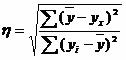 , where ∑(y avg -y x) 2 = ∑(y i -y avg) 2 - ∑(y i -y x) 2 = 138000 - 46000 = 92,000.
η 2 = 92,000/138000 = 0.67, η = 0.816 (0.7< η < 0.9 - связь между X и Y высокая).
R 2 = 1 - 46000/138000 = 0.67, F = 0.67/(1-0.67)x(25 - 1 - 1) = 46. F table (1; 23) = 4.27
Since the actual value F > Ftable, the found estimate of the regression equation is statistically reliable.
Answer: For the significance of the entire model as a whole, F-statistics (Fisher's test) are used.1. History of the development of the criterion
2. What is Fisher's exact test used for?
3. In what cases can Fisher's exact test be used?
A two-tailed test evaluates frequency differences in two directions. That is, the likelihood of both a higher and lower frequency of the phenomenon in the experimental group compared to the control group is assessed.4. How to calculate Fisher's exact test?
5. How to interpret the value of Fisher's exact test?


