Actions with matrices. Finding the inverse matrix

Matrices in mathematics are one of the most important objects of practical importance. Often an excursion into the theory of matrices begins with the words: “A matrix is a rectangular table...”. We will start this excursion from a slightly different direction.

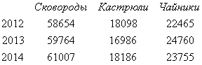
Phone books of any size and with any amount of subscriber data are nothing more than matrices. Such matrices look approximately like this:

It is clear that we all use such matrices almost every day. These matrices come with a different number of rows (they vary like a directory issued by a telephone company, which can have thousands, hundreds of thousands and even millions of lines, and a new notebook you just started, which has less than ten lines) and columns (a directory of officials of some kind). some organization in which there may be columns such as position and office number and your same address book, where there may not be any data except the name, and thus there are only two columns in it - name and telephone number).

All sorts of matrices can be added and multiplied, as well as other operations can be performed on them, but there is no need to add and multiply telephone directories, there is no benefit from this, and besides, you can use your mind.

But many matrices can and should be added and multiplied and thus solve various pressing problems. Below are examples of such matrices.

Matrices in which the columns are the production of units of a particular type of product, and the rows are the years in which the production of this product is recorded:

You can add matrices of this type, which take into account the output of similar products by different enterprises, in order to obtain summary data for the industry.

Or matrices consisting, for example, of one column, in which the rows are the average cost of a particular type of product:

The last two types of matrices can be multiplied, and the result is a row matrix containing the cost of all types of products by year.

Matrices, basic definitions

A rectangular table consisting of numbers arranged in m lines and n columns is called mn-matrix (or simply matrix ) and is written like this:

(1)

In matrix (1) the numbers are called its elements (as in the determinant, the first index means the number of the row, the second – the column at the intersection of which the element stands; i = 1, 2, ..., m; j = 1, 2, n).

The matrix is called rectangular , If .

If m = n, then the matrix is called square , and the number n is its in order .

Determinant of a square matrix A is a determinant whose elements are the elements of a matrix A. It is indicated by the symbol | A|.

The square matrix is called not special (or non-degenerate , non-singular ), if its determinant is not zero, and special (or degenerate , singular ) if its determinant is zero.

The matrices are called equal , if they have the same number of rows and columns and all corresponding elements match.

The matrix is called null , if all its elements are equal to zero. We will denote the zero matrix by the symbol 0 or .

For example,

Matrix-row (or lowercase ) is called 1 n-matrix, and matrix-column (or columnar ) – m 1-matrix.

Matrix A", which is obtained from the matrix A swapping rows and columns in it is called transposed relative to the matrix A. Thus, for matrix (1) the transposed matrix is

Matrix transition operation A" transposed with respect to the matrix A, is called matrix transposition A. For mn-matrix transposed is nm-matrix.

The matrix transposed with respect to the matrix is A, that is

(A")" = A .

Example 1. Find matrix A" , transposed with respect to the matrix

and find out whether the determinants of the original and transposed matrices are equal.

Main diagonal A square matrix is an imaginary line connecting its elements, for which both indices are the same. These elements are called diagonal .

A square matrix in which all elements off the main diagonal are equal to zero is called diagonal . Not all diagonal elements of a diagonal matrix are necessarily nonzero. Among them there may be equal to zero.

A square matrix in which the elements on the main diagonal are equal to the same number, non-zero, and all others are equal to zero, is called scalar matrix .

Identity matrix is called a diagonal matrix in which all diagonal elements are equal to one. For example, the third-order identity matrix is the matrix

Example 2. Given matrices:

Solution. Let us calculate the determinants of these matrices. Using the triangle rule, we find

Matrix determinant B let's calculate using the formula

We easily get that

Therefore, the matrices A and are non-singular (non-degenerate, non-singular), and the matrix B– special (degenerate, singular).

The determinant of the identity matrix of any order is obviously equal to one.

Solve the matrix problem yourself, and then look at the solution

Example 3. Given matrices

Determine which of them are non-singular (non-degenerate, non-singular).

Application of matrices in mathematical and economic modeling

Structured data about a particular object is simply and conveniently recorded in the form of matrices. Matrix models are created not only to store this structured data, but also to solve various problems with this data using linear algebra.

Thus, a well-known matrix model of the economy is the input-output model, introduced by the American economist of Russian origin Vasily Leontiev. This model is based on the assumption that the entire production sector of the economy is divided into n clean industries. Each industry produces only one type of product, and different industries produce different products. Due to this division of labor between industries, there are inter-industry connections, the meaning of which is that part of the production of each industry is transferred to other industries as a production resource.

Product volume i-th industry (measured by a specific unit of measurement), which was produced during the reporting period, is denoted by and is called full output i-th industry. Issues can be conveniently placed in n-component row of the matrix.

Number of units i-industry that needs to be spent j-industry for the production of a unit of its output is designated and called the direct cost coefficient.

Solving matrices– a concept that generalizes operations on matrices. A mathematical matrix is a table of elements. A table like this, which has m rows and n columns, is said to be an m by n matrix.
General view of the matrix

Main elements of the matrix:
Main diagonal. It is made up of the elements a 11, a 22…..a mn
Side diagonal. It is composed of the elements a 1n, and 2n-1.....a m1.
Before moving on to solving matrices, let’s consider the main types of matrices:
Square– in which the number of rows is equal to the number of columns (m=n)
Zero – all elements of this matrix are equal to 0.
Transposed matrix- matrix B obtained from the original matrix A by replacing rows with columns.
Single– all elements of the main diagonal are equal to 1, all others are 0.
inverse matrix- a matrix, when multiplied by which the original matrix results in the identity matrix.
The matrix can be symmetrical with respect to the main and secondary diagonals. That is, if a 12 = a 21, a 13 = a 31,….a 23 = a 32…. a m-1n = a mn-1 . then the matrix is symmetrical about the main diagonal. Only square matrices are symmetrical.
Now let's move directly to the question of how to solve matrices.

Matrix addition.

Matrices can be added algebraically if they have the same dimension. To add matrix A with matrix B, you need to add the element of the first row of the first column of matrix A with the first element of the first row of matrix B, the element of the second column of the first row of matrix A with the element of the second column of the first row of matrix B, etc.
Properties of addition
A+B=B+A
(A+B)+C=A+(B+C)

Matrix multiplication.

Matrices can be multiplied if they are consistent. Matrices A and B are considered consistent if the number of columns of matrix A is equal to the number of rows of matrix B.
If A is of dimension m by n, B is of dimension n by k, then the matrix C=A*B will be of dimension m by k and will be composed of elements

Where C 11 is the sum of pairwise products of the elements of a row of matrix A and a column of matrix B, that is, the element is the sum of the product of an element of the first column of the first row of matrix A with an element of the first column of the first row of matrix B, an element of the second column of the first row of matrix A with an element of the first column of the second row matrices B, etc.
When multiplying, the order of multiplication is important. A*B is not equal to B*A.

Finding the determinant.

Any square matrix can generate a determinant or a determinant. Writes det. Or | matrix elements |
For matrices of dimension 2 by 2. Determine there is a difference between the product of the elements of the main and the elements of the secondary diagonal.

For matrices with dimensions of 3 by 3 or more. The operation of finding the determinant is more complicated.
Let's introduce the concepts:
Element minor– is the determinant of a matrix obtained from the original matrix by crossing out the row and column of the original matrix in which this element was located.
Algebraic complement element of a matrix is the product of the minor of this element by -1 to the power of the sum of the row and column of the original matrix in which this element was located.
The determinant of any square matrix is equal to the sum of the product of the elements of any row of the matrix and their corresponding algebraic complements.

Matrix inversion

Matrix inversion is the process of finding the inverse of a matrix, the definition of which we gave at the beginning. The inverse matrix is denoted in the same way as the original one with the addition of degree -1.
Find the inverse matrix using the formula.
A -1 = A * T x (1/|A|)
Where A * T is the Transposed Matrix of Algebraic Complements.

We made examples of solving matrices in the form of a video tutorial

:

If you want to figure it out, be sure to watch it.

These are the basic operations for solving matrices. If you have additional questions about how to solve matrices, feel free to write in the comments.

If you still can’t figure it out, try contacting a specialist.

A mathematical matrix is a table of ordered elements. The dimensions of this table are determined by the number of rows and columns in it. As for solving matrices, it refers to the huge number of operations that are performed on these same matrices. Mathematicians distinguish several types of matrices. For some of them, general decision rules apply, while for others they do not. For example, if the matrices have the same dimension, then they can be added, and if they are consistent with each other, then they can be multiplied. To solve any matrix, it is necessary to find a determinant. In addition, matrices are subject to transposition and the finding of minors in them. So let's look at how to solve matrices.

The order of solving matrices

First we write down the given matrices. We count how many rows and columns they have. If the number of rows and columns is the same, then such a matrix is called square. If every element of the matrix is equal to zero, then such a matrix is zero. The next thing we do is find the main diagonal of the matrix. The elements of such a matrix are located from the lower right corner to the upper left. The second diagonal in the matrix is a secondary one. Now you need to transpose the matrix. To do this, it is necessary to replace the row elements in each of the two matrices with the corresponding column elements. For example, the element under a21 will turn out to be the element a12, or vice versa. Thus, after this procedure a completely different matrix should appear.

If the matrices have exactly the same dimensions, then they can be easily added. To do this, we take the first element of the first matrix a11 and add it with a similar element of the second matrix b11. We write what happens as a result in the same position, only in a new matrix. Now we add all the other elements of the matrix in the same way until we get a new completely different matrix. Let's look at a few more ways to solve matrices.

Options for working with matrices

We can also determine whether the matrices are consistent. To do this, we need to compare the number of rows in the first matrix with the number of columns in the second matrix. If they turn out to be equal, you can multiply them. To do this, we pairwise multiply a row element of one matrix by a similar column element of another matrix. Only after this will it be possible to calculate the sum of the resulting products. Based on this, the initial element of the matrix that should be obtained as a result will be equal to g11 = a11* b11 + a12*b21 + a13*b31 + … + a1m*bn1. Once all the products have been added and multiplied, you can fill out the final matrix.

When solving matrices, you can also find their determinant and determinant for each. If the matrix is square and has a dimension of 2 by 2, then the determinant can be found as the difference of all the products of the elements of the main and secondary diagonals. If the matrix is already three-dimensional, then the determinant can be found by applying the following formula. D = a11* a22*a33 + a13* a21*a32 + a12* a23*a31 - a21* a12*a33 - a13* a22*a31 - a11* a32*a23.

To find the minor of a given element, you need to cross out the column and row where this element is located. After this, find the determinant of this matrix. He will be the corresponding minor. A similar decision matrix method was developed several decades ago in order to increase the reliability of the result by dividing the problem into subproblems. So, solving matrices is not that difficult if you know the basic math operations.

Instructions

The number of columns and rows is specified dimension matrices. Eg, dimension yu 5x6 has 5 rows and 6 columns. In general, dimension matrices written in the form m×n, where the number m indicates the number of rows, n – columns.

If the array has dimension m×n, it can be multiplied by an n×l array. Number of columns first matrices must be equal to the number of rows of the second, otherwise the multiplication operation will not be defined.

Dimension matrices indicates the number of equations in the system and the number of variables. The number of rows coincides with the number of equations, and each column has its own variable. The solution to a system of linear equations is “written” in operations on matrices. Thanks to the matrix recording system, high order systems are possible.

If the number of rows is equal to the number of columns, the matrix is square. In it you can distinguish the main and secondary diagonals. The main one goes from the upper left corner to the lower right, the secondary one goes from the upper right to the lower left.

Arrays dimension yu m×1 or 1×n are vectors. You can also represent any row and any column of an arbitrary table as a vector. For such matrices, all operations on vectors are defined.

In programming, two indexes are specified for a rectangular table, one of which runs through the entire row, the other – the length of the column. In this case, the cycle for one index is placed inside the cycle for another, due to which the sequential passage of the entire dimension matrices.

Matrices is an effective way of representing numerical information. The solution to any system of linear equations can be written in the form of a matrix (a rectangle made up of numbers). The ability to multiply matrices is one of the most important skills taught in Linear Algebra courses in higher education.

You will need

Calculator

Instructions

To check this condition, the easiest way is to use the following algorithm - write the dimension of the first matrix as (a*b). Then the second dimension is (c*d). If b=c - the matrices are commensurate, they can be multiplied.

Next, perform the multiplication itself. Remember - when you multiply two matrices, you get a matrix. That is, the problem of multiplication is reduced to the problem of finding a new one, with dimension (a*d). In SI, the matrix multiplication problem looks like this:
void matrixmult(int m1[n], int m1_row, int m1_col, int m2[n], int m2_row, int m2_col, int m3[n], int m3_row, int m3_col)
( for (int i = 0; i< m3_row; i++)
for (int j = 0; j< m3_col; j++)
m3[i][j]=0;
for (int k = 0; k< m2_col; k++)
for (int i = 0; i< m1_row; i++)
for (int j = 0; j< m1_col; j++)
m3[i][k] += m1[i][j] * m2[j][k];
}

Simply put, a new matrix is the sum of the products of the row elements of the first matrix and the column elements of the second matrix. If you are the element of the third matrix with number (1;2), then you should simply multiply the first row of the first matrix by the second column of the second. To do this, consider the initial amount to be zero. Next, multiply the first element of the first row by the first element of the second column, adding the value to the sum. You do this: multiply the i-th element of the first row by the i-th element of the second column and add the results to the sum until the row ends. The total amount will be the required element.

After you have found all the elements of the third matrix, write it down. You have found work matrices

Sources:

The main mathematical portal of Russia in 2019
how to find the product of matrices in 2019

A mathematical matrix is an ordered table of elements. Dimension matrices is determined by the number of its rows m and columns n. By solving matrices we mean a set of generalizing operations performed on matrices. There are several types of matrices; a number of operations cannot be applied to some of them. There is an addition operation for matrices with the same dimension. The product of two matrices can only be found if they are consistent. For anyone matrices determinant is determined. You can also transpose the matrix and determine the minor of its elements.

Instructions

Write down the given ones. Determine their size. To do this, count the number of columns n and rows m. If for one matrices m = n, the matrix is considered square. If all elements matrices are equal to zero – the matrix is zero. Determine the main diagonal of the matrices. Its elements are located in the upper left corner matrices to the bottom right. Second, reverse diagonal matrices is a side effect.

Perform matrix transposition. To do this, replace the row elements in each with column elements relative to the main diagonal. Element a21 will become element a12 matrices and vice versa. As a result, from each initial matrices you will get a new transposed matrix.

Add up the given matrices, if they have the same dimension m x n. To do this, take the first matrices a11 and add it to the second similar element b11 matrices. Write the result of the addition into a new one in the same position. Then add elements a12 and b12 of both matrices. Thus, fill in all the rows and columns of the summarizing matrices.

Determine whether the given matrices agreed upon. To do this, compare the number of lines n in the first matrices and the number of columns m second matrices. If they are equal, do the matrix product. To do this, multiply each element of the first row in pairs matrices to the corresponding element of the second column matrices. Then find the sum of these products. Thus, the first element of the resulting matrices g11 = a11* b11 + a12*b21 + a13*b31 + … + a1m*bn1. Perform multiplication and addition of all products and fill in the resulting matrix G.

Find the determinant or determinant for each given matrices. For matrices of the second - with dimensions 2 by 2 - the determinant is found as the product of the elements of the main and secondary diagonals matrices. For three-dimensional matrices determinant: D = a11* a22*a33 + a13* a21*a32 + a12* a23*a31 - a21* a12*a33 - a13* a22*a31 - a11* a32*a23.

Sources:

matrix how to solve

Matrices represent a set of rows and columns at the intersection of which are the matrix elements. Matrices widely used to solve various equations. One of the basic algebraic operations on matrices is matrix addition. How to add matrices?

Instructions

Only one-dimensional matrices can be added. If one has m rows and n columns, then the other matrix must also have m rows and n columns. Make sure that the folding dies are the same size.

If the presented matrices are the same size, that is, they allow the algebraic operation of addition, then the matrix is the same size. To do it, you need to add in pairs all the elements of two that are in the same places. Take the first matrix, located in the first row and first column. Add it to the element of the second matrix located in the same place. Enter the result into the element of the first row of the column of the summary matrix. Do this operation with all elements.

The addition of three or more matrices is reduced to the addition of two matrices. For example, to find the sum of matrices A+B+C, first find the sum of matrices A and B, then add the resulting sum to matrix C.

Video on the topic

The matrices, which are incomprehensible at first glance, are actually not so complex. They find wide practical application in economics and accounting. Matrices look like tables, each column and row containing a number, function or any other value. There are several types of matrices.

Instructions

In order to learn the matrix, get acquainted with its basic concepts. The defining elements of a matrix are its diagonals and its side diagonals. Home starts with the element in the first row, first column and continues to the element in the last column, last row (that is, it goes from left to right). The side diagonal begins on the contrary in the first row, but in the last column and continues to the element that has the coordinates of the first column and the last row (goes from right to left).

To move on to the following definitions and algebraic operations with matrices, study the types of matrices. The simplest ones are square, unit, zero and inverse. The number of columns and rows matches. The transposed matrix, let's call it B, is obtained from matrix A by replacing the columns with rows. In unit, all the elements of the main diagonal are ones, and the others are zeros. And in zero, even the elements of the diagonals are zero. The inverse matrix is the one on which the original matrix comes to the identity form.

Also, the matrix can be symmetrical about the main or secondary axes. That is, an element having coordinates a(1;2), where 1 is the row number and 2 is the column number, is equal to a(2;1). A(3;1)=A(1;3) and so on. Matched matrices are those where the number of columns of one is equal to the number of rows of another (such matrices can be multiplied).

The main actions that can be performed with matrices are addition, multiplication and finding the determinant. If the matrices are the same size, that is, they have an equal number of rows and columns, then they can be added. It is necessary to add elements that are in the same places in the matrices, that is, add a (m; n) with c in (m; n), where m and n are the corresponding coordinates of the column and row. When adding matrices, the main rule of ordinary arithmetic addition applies - when the places of the terms are changed, the sum does not change. Thus, if instead of a simple element a

In this topic we will consider the concept of a matrix, as well as types of matrices. Since there are a lot of terms in this topic, I will add a brief summary to make it easier to navigate the material.

Definition of a matrix and its element. Notation.

Matrix is a table of $m$ rows and $n$ columns. The elements of a matrix can be objects of a completely different nature: numbers, variables or, for example, other matrices. For example, the matrix $\left(\begin(array) (cc) 5 & 3 \\ 0 & -87 \\ 8 & 0 \end(array) \right)$ contains 3 rows and 2 columns; its elements are integers. The matrix $\left(\begin(array) (cccc) a & a^9+2 & 9 & \sin x \\ -9 & 3t^2-4 & u-t & 8\end(array) \right)$ contains 2 rows and 4 columns.

Different ways to write matrices: show\hide

The matrix can be written not only in round, but also in square or double straight brackets. That is, the entries below mean the same matrix:

$$ \left(\begin(array) (cc) 5 & 3 \\ 0 & -87 \\ 8 & 0 \end(array) \right);\;\; \left[ \begin(array) (cc) 5 & 3 \\ 0 & -87 \\ 8 & 0 \end(array) \right]; \;\; \left \Vert \begin(array) (cc) 5 & 3 \\ 0 & -87 \\ 8 & 0 \end(array) \right \Vert $$

The product $m\times n$ is called matrix size. For example, if a matrix contains 5 rows and 3 columns, then we speak of a matrix of size $5\times 3$. The matrix $\left(\begin(array)(cc) 5 & 3\\0 & -87\\8 & 0\end(array)\right)$ has size $3 \times 2$.

Typically, matrices are denoted by capital letters of the Latin alphabet: $A$, $B$, $C$ and so on. For example, $B=\left(\begin(array) (ccc) 5 & 3 \\ 0 & -87 \\ 8 & 0 \end(array) \right)$. Line numbering goes from top to bottom; columns - from left to right. For example, the first row of matrix $B$ contains elements 5 and 3, and the second column contains elements 3, -87, 0.

Elements of matrices are usually denoted in small letters. For example, the elements of the matrix $A$ are denoted by $a_(ij)$. The double index $ij$ contains information about the position of the element in the matrix. The number $i$ is the row number, and the number $j$ is the column number, at the intersection of which is the element $a_(ij)$. For example, at the intersection of the second row and the fifth column of the matrix $A=\left(\begin(array) (cccccc) 51 & 37 & -9 & 0 & 9 & 97 \\ 1 & 2 & 3 & 41 & 59 & 6 \ \ -17 & -15 & -13 & -11 & -8 & -5 \\ 52 & 31 & -4 & -1 & 17 & 90 \end(array) \right)$ element $a_(25)= $59:

In the same way, at the intersection of the first row and the first column we have the element $a_(11)=51$; at the intersection of the third row and the second column - the element $a_(32)=-15$ and so on. Note that the entry $a_(32)$ reads “a three two”, but not “a thirty two”.

To abbreviate the matrix $A$, the size of which is $m\times n$, the notation $A_(m\times n)$ is used. You can write it in a little more detail:

$$ A_(m\times n)=(a_(ij)) $$

where the notation $(a_(ij))$ denotes the elements of the matrix $A$. In its fully expanded form, the matrix $A_(m\times n)=(a_(ij))$ can be written as follows:

$$ A_(m\times n)=\left(\begin(array)(cccc) a_(11) & a_(12) & \ldots & a_(1n) \\ a_(21) & a_(22) & \ldots & a_(2n) \\ \ldots & \ldots & \ldots & \ldots \\ a_(m1) & a_(m2) & \ldots & a_(mn) \end(array) \right) $$

Let's introduce another term - equal matrices.

Two matrices of the same size $A_(m\times n)=(a_(ij))$ and $B_(m\times n)=(b_(ij))$ are called equal, if their corresponding elements are equal, i.e. $a_(ij)=b_(ij)$ for all $i=\overline(1,m)$ and $j=\overline(1,n)$.

Explanation for the entry $i=\overline(1,m)$: show\hide

The notation "$i=\overline(1,m)$" means that the parameter $i$ varies from 1 to m. For example, the notation $i=\overline(1,5)$ indicates that the parameter $i$ takes the values 1, 2, 3, 4, 5.

So, for matrices to be equal, two conditions must be met: coincidence of sizes and equality of the corresponding elements. For example, the matrix $A=\left(\begin(array)(cc) 5 & 3\\0 & -87\\8 & 0\end(array)\right)$ is not equal to the matrix $B=\left(\ begin(array)(cc) 8 & -9\\0 & -87 \end(array)\right)$ because matrix $A$ has size $3\times 2$ and matrix $B$ has size $2\times $2. Also, matrix $A$ is not equal to matrix $C=\left(\begin(array)(cc) 5 & 3\\98 & -87\\8 & 0\end(array)\right)$, since $a_( 21)\neq c_(21)$ (i.e. $0\neq 98$). But for the matrix $F=\left(\begin(array)(cc) 5 & 3\\0 & -87\\8 & 0\end(array)\right)$ we can safely write $A=F$ because both the sizes and the corresponding elements of the matrices $A$ and $F$ coincide.

Example No. 1

Determine the size of the matrix $A=\left(\begin(array) (ccc) -1 & -2 & 1 \\ 5 & 9 & -8 \\ -6 & 8 & 23 \\ 11 & -12 & -5 \ \4 & 0 & -10 \\ \end(array) \right)$. Indicate what the elements $a_(12)$, $a_(33)$, $a_(43)$ are equal to.

This matrix contains 5 rows and 3 columns, so its size is $5\times 3$. You can also use the notation $A_(5\times 3)$ for this matrix.

Element $a_(12)$ is at the intersection of the first row and second column, so $a_(12)=-2$. Element $a_(33)$ is at the intersection of the third row and third column, so $a_(33)=23$. Element $a_(43)$ is at the intersection of the fourth row and third column, so $a_(43)=-5$.

Answer: $a_(12)=-2$, $a_(33)=23$, $a_(43)=-5$.

Types of matrices depending on their size. Main and secondary diagonals. Matrix trace.

Let a certain matrix $A_(m\times n)$ be given. If $m=1$ (the matrix consists of one row), then the given matrix is called matrix-row. If $n=1$ (the matrix consists of one column), then such a matrix is called matrix-column. For example, $\left(\begin(array) (ccccc) -1 & -2 & 0 & -9 & 8 \end(array) \right)$ is a row matrix, and $\left(\begin(array) (c) -1 \\ 5 \\ 6 \end(array) \right)$ is a column matrix.

If the matrix $A_(m\times n)$ satisfies the condition $m\neq n$ (i.e., the number of rows is not equal to the number of columns), then it is often said that $A$ is a rectangular matrix. For example, the matrix $\left(\begin(array) (cccc) -1 & -2 & 0 & 9 \\ 5 & 9 & 5 & 1 \end(array) \right)$ has size $2\times 4$, those. contains 2 rows and 4 columns. Since the number of rows is not equal to the number of columns, this matrix is rectangular.

If the matrix $A_(m\times n)$ satisfies the condition $m=n$ (i.e., the number of rows is equal to the number of columns), then $A$ is said to be a square matrix of order $n$. For example, $\left(\begin(array) (cc) -1 & -2 \\ 5 & 9 \end(array) \right)$ is a second-order square matrix; $\left(\begin(array) (ccc) -1 & -2 & 9 \\ 5 & 9 & 8 \\ 1 & 0 & 4 \end(array) \right)$ is a third-order square matrix. In general, the square matrix $A_(n\times n)$ can be written as follows:

$$ A_(n\times n)=\left(\begin(array)(cccc) a_(11) & a_(12) & \ldots & a_(1n) \\ a_(21) & a_(22) & \ldots & a_(2n) \\ \ldots & \ldots & \ldots & \ldots \\ a_(n1) & a_(n2) & \ldots & a_(nn) \end(array) \right) $$

The elements $a_(11)$, $a_(22)$, $\ldots$, $a_(nn)$ are said to be on main diagonal matrices $A_(n\times n)$. These elements are called main diagonal elements(or just diagonal elements). The elements $a_(1n)$, $a_(2 \; n-1)$, $\ldots$, $a_(n1)$ are on side (minor) diagonal; they are called side diagonal elements. For example, for the matrix $C=\left(\begin(array)(cccc)2&-2&9&1\\5&9&8& 0\\1& 0 & 4 & -7 \\ -4 & -9 & 5 & 6\end(array) \right)$ we have:

The elements $c_(11)=2$, $c_(22)=9$, $c_(33)=4$, $c_(44)=6$ are the main diagonal elements; elements $c_(14)=1$, $c_(23)=8$, $c_(32)=0$, $c_(41)=-4$ are side diagonal elements.

The sum of the main diagonal elements is called followed by the matrix and is denoted by $\Tr A$ (or $\Sp A$):

$$ \Tr A=a_(11)+a_(22)+\ldots+a_(nn) $$

For example, for the matrix $C=\left(\begin(array) (cccc) 2 & -2 & 9 & 1\\5 & 9 & 8 & 0\\1 & 0 & 4 & -7\\-4 & -9 & 5 & 6 \end(array)\right)$ we have:

$$ \Tr C=2+9+4+6=21. $$

The concept of diagonal elements is also used for non-square matrices. For example, for the matrix $B=\left(\begin(array) (ccccc) 2 & -2 & 9 & 1 & 7 \\ 5 & -9 & 8 & 0 & -6 \\ 1 & 0 & 4 & - 7 & -6 \end(array) \right)$ the main diagonal elements will be $b_(11)=2$, $b_(22)=-9$, $b_(33)=4$.

Types of matrices depending on the values of their elements.

If all elements of the matrix $A_(m\times n)$ are equal to zero, then such a matrix is called null and is usually denoted by the letter $O$. For example, $\left(\begin(array) (cc) 0 & 0 \\ 0 & 0 \\ 0 & 0 \end(array) \right)$, $\left(\begin(array) (ccc) 0 & 0 & 0 \\ 0 & 0 & 0 \\ 0 & 0 & 0 \end(array) \right)$ - zero matrices.

Let the matrix $A_(m\times n)$ have the following form:

Then this matrix is called trapezoidal. It may not contain zero rows, but if they exist, they are located at the bottom of the matrix. In a more general form, a trapezoidal matrix can be written as follows:

Again, trailing null lines are not required. Those. Formally, we can distinguish the following conditions for a trapezoidal matrix:

All elements below the main diagonal are zero.
All elements from $a_(11)$ to $a_(rr)$ lying on the main diagonal are not equal to zero: $a_(11)\neq 0, \; a_(22)\neq 0, \ldots, a_(rr)\neq 0$.
Either all elements of the last $m-r$ rows are zero, or $m=r$ (i.e. there are no zero rows at all).

Examples of trapezoidal matrices:

Let's move on to the next definition. The matrix $A_(m\times n)$ is called stepped, if it satisfies the following conditions:

For example, step matrices would be:

For comparison, the matrix $\left(\begin(array) (cccc) 2 & -2 & 0 & 1\\0 & 0 & 8 & 7\\0 & 0 & 4 & -7\\0 & 0 & 0 & 0 \end(array)\right)$ is not echelon because the third row has the same zero part as the second row. That is, the principle “the lower the line, the larger the zero part” is violated. I will add that a trapezoidal matrix is a special case of a stepped matrix.

Let's move on to the next definition. If all elements of a square matrix located under the main diagonal are equal to zero, then such a matrix is called upper triangular matrix. For example, $\left(\begin(array) (cccc) 2 & -2 & 9 & 1 \\ 0 & 9 & 8 & 0 \\ 0 & 0 & 4 & -7 \\ 0 & 0 & 0 & 6 \end(array) \right)$ is an upper triangular matrix. Note that the definition of an upper triangular matrix does not say anything about the values of the elements located above the main diagonal or on the main diagonal. They can be zero or not - it doesn't matter. For example, $\left(\begin(array) (ccc) 0 & 0 & 9 \\ 0 & 0 & 0\\ 0 & 0 & 0 \end(array) \right)$ is also an upper triangular matrix.

If all elements of a square matrix located above the main diagonal are equal to zero, then such a matrix is called lower triangular matrix. For example, $\left(\begin(array) (cccc) 3 & 0 & 0 & 0 \\ -5 & 1 & 0 & 0 \\ 8 & 2 & 1 & 0 \\ 5 & 4 & 0 & 6 \ end(array) \right)$ - lower triangular matrix. Note that the definition of a lower triangular matrix does not say anything about the values of the elements located under or on the main diagonal. They may be zero or not - it doesn't matter. For example, $\left(\begin(array) (ccc) -5 & 0 & 0 \\ 0 & 0 & 0\\ 0 & 0 & 9 \end(array) \right)$ and $\left(\begin (array) (ccc) 0 & 0 & 0 \\ 0 & 0 & 0\\ 0 & 0 & 0 \end(array) \right)$ are also lower triangular matrices.

The square matrix is called diagonal, if all elements of this matrix that do not lie on the main diagonal are equal to zero. Example: $\left(\begin(array) (cccc) 3 & 0 & 0 & 0 \\ 0 & -2 & 0 & 0 \\ 0 & 0 & 0 & 0 \\ 0 & 0 & 0 & 6 \ end(array)\right)$. The elements on the main diagonal can be anything (equal to zero or not) - it doesn't matter.

The diagonal matrix is called single, if all elements of this matrix located on the main diagonal are equal to 1. For example, $\left(\begin(array) (cccc) 1 & 0 & 0 & 0 \\ 0 & 1 & 0 & 0 \\ 0 & 0 & 1 & 0 \\ 0 & 0 & 0 & 1 \end(array)\right)$ - fourth-order identity matrix; $\left(\begin(array) (cc) 1 & 0 \\ 0 & 1 \end(array)\right)$ is the second-order identity matrix.