Protecting cells in Excel from changing, editing and entering erroneous data. How to protect cells in Excel from editing

This article will discuss how to protect a cell in Excel from changes. Fortunately, this option is present in this spreadsheet editor. And you can easily protect all the data you enter from someone else’s interference. Also protecting cells is a good way to save yourself from yourself. By protecting the cells in which formulas are entered, you will not accidentally delete them.

Select the required range of cells

Now the first method will be provided on how to protect cells in Excel from changes. It is, of course, not much different from the second one, which will be described later, but it cannot be missed.

So, in order to protect table cells from corrections, you need to do the following:

Select the entire table. The easiest way to do this is by clicking on a special button, which is located at the intersection of the vertical (row numbering) and horizontal (column designation). However, you can also use hotkeys by pressing CTRL+A.

Press the right mouse button (RMB).

Select "Format Cells" from the menu.

In the window that appears, go to the "Protection" tab.

Uncheck the "Protected cell" checkbox.

Click OK.

So, we've just removed the ability to protect all cells in a table. This is necessary in order to designate only a range or one cell. To do this you need:

Select the required cells using normal stretching while holding down the left mouse button (LMB).

Press RMB.

Select "Format Cells" from the menu again.

Go to "Protection".

Check the box next to "Protected cell".

Click OK.

We put protection on selected cells

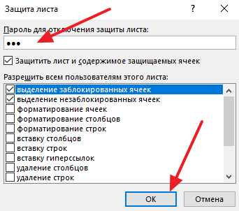
We indicated to the program which cells we want to protect from changes. But this is not enough for them to become protected. To achieve this goal, you need to enable sheet protection in Excel. For this:

Click on the "File" tab.

In the menu, go to the "Information" section.

Click on the "Protect Book" icon.

From the menu, select Protect Current Sheet.

A window will appear in which you need to make settings. Follow the guide:

Never uncheck the “Protect sheet and contents of protected cells” checkbox.

In the window located just below, you can make more flexible settings, but by default it is set so that no one can change the parameters.

Enter your password in the appropriate field. It can be of any length, but remember that the more complex and longer it is, the more reliable it is.

Click OK.

After the manipulations have been completed, you will be asked to re-enter your password for all changes to take effect. Now you know the first way to protect a cell in Excel from changes.

Second way

The second way to protect a cell in Excel from changes, as mentioned above, is not much different from the first. Here are detailed instructions.

Just like last time, remove cell protection from the entire table and place it in the desired area.

Go to "Review".

Click on the "Protect Sheet" button, which is located in the "Changes" tool group.

After this, a familiar window will appear in which you need to set protection parameters. Enter the password in the same way, select the necessary options, check the box next to “Protect the sheet and contents of protected cells” and click OK.

Filling out Excel tables is a fairly routine process that can lead to errors. Often, when entering data into a table, users accidentally change other cells and have to spend even more time correcting these errors.

In this article we will talk about how to protect Excel cells from editing. The article will be useful for current versions of Excel, such as Excel 2007, 2010, 2013 and 2016.

The problem is that Excel does not have the ability to protect individual cells from editing. There are no functions to directly implement this idea. But there is one trick that allows you to get almost the same result. You can protect an entire Excel sheet from changes, but still be able to edit individual cells.

To implement this method, you need to select those cells in which you want to leave the ability to edit data, right-click on them and select “Format Cells” in the menu that opens.

As a result, the “Format Cells” window will open in front of you. Here you need to go to the “Protection” tab, uncheck the “Protected cell” function and save the settings by clicking on the “OK” button.

After this, you need to right-click on the sheet name at the bottom of the page and select “Protect Sheet” from the menu that opens.

Then enter the password again to confirm and click on the “OK” button again. An important point: it is better not to forget the password, otherwise you will not be able to remove the protection from the sheet later.

That's all, you have protected all the cells of this Excel sheet, of course, except for those for which you have disabled the “Protected Cell” function. Now, when working with this Excel sheet, the user will not be able to change any unnecessary data since only individual cells will be available for editing.

If in the future you come to remove protection from this sheet, then this is done in a similar way. Right-click on the sheet name, select “Unprotect” and enter the password. Without a password, you will not be able to remove protection from the sheet.

It should be noted that even if the sheet is protected, the user still has the ability to change the name and delete this sheet. In order to avoid such problems, you need to protect the entire Excel workbook. To do this, go to the “Review” tab, click on the “Protect Book” button and enter the password twice, as was shown above.

By adding protection to the entire workbook, you will prohibit the user from any operations with the sheets and structure of the document, which will significantly increase the security of work.

Data in Excel can be protected from outside interference. This is important because sometimes you spend a lot of time and effort creating a pivot table or volumetric array, and another person accidentally or intentionally changes or completely deletes all your work.

Let's look at ways to protect an Excel document and its individual elements.

Protecting an Excel cell from modification

How to protect a cell in Excel? By default, all cells in Excel are protected. This is easy to check: right-click on any cell and select FORMAT CELLS - PROTECTION. We see that the PROTECTED CELL checkbox is checked. But this does not mean that they are already protected from changes.

Why do we need this information? The fact is that Excel does not have a function that allows you to protect a single cell. You can choose to protect a sheet, and then all cells on it will be protected from editing and other interference. On the one hand, this is convenient, but what if we need to protect not all cells, but only some?

Let's look at an example. We have a simple table with data. We need to send this table to the branches so that the stores fill out the QUANTITY SOLD column and send it back. To avoid making any changes to other cells, we will protect them.

First, let's release from protection those cells where branch employees will make changes. Select D4:D11, right-click to open the menu, select CELL FORMAT and uncheck the PROTECTED CELL item.

Now select the REVIEW – PROTECT SHEET tab. A window appears with 2 checkboxes. We remove the first of them in order to exclude any intervention by branch employees other than filling out the QUANTITY SOLD column. Create a password and click OK.

Attention! Don't forget your password!

Now, unauthorized persons will only be able to enter a value in the range D4:D11. Because We have limited all other actions, no one can even change the background color. All formatting tools on the top toolbar are disabled. Those. they do not work.

Protecting an Excel workbook from editing

If several people work on one computer, then it is advisable to protect your documents from editing by third parties. You can protect not only individual sheets, but also the entire book.

When the book is protected, outsiders will be able to open the document, see the written data, but rename the sheets, insert a new one, change their location, etc. Let's try.

We keep the previous formatting. Those. We still only allow changes to be made to the QUANTITY SOLD column. To protect a book completely, on the REVIEW tab, select PROTECT BOOK. Leave the checkbox next to the STRUCTURE item and come up with a password.

Now, if we try to rename the sheet, it won't work. All commands are gray: they do not work.

The protection is removed from the sheet and book using the same buttons. When removed, the system will require the same password.

In this article I will tell you how to protect cells in Excel from changes and editing. Cell protection may mean that users who open your file will not be able to edit cell values ​​or see formulas.

Before we figure out how to set up protection, it is important to understand how cell protection works in Excel. By default, all cells in Excel are already locked, but in fact, access to them will be limited after you enter a password and access restriction conditions in the sheet protection settings.

How to protect all cells in an Excel file

If you want to protect absolutely all cells in your Excel file from editing and changes, do the following:

• Go to the “ Review” on the toolbar => in the subsection “ Protection” click on the icon “ Protect sheet “:

• In the pop-up window, make sure the checkbox next to ““ is checked:

• Enter the password in the ““ field if you want only those users to whom you have shared the password to be able to remove the protection:

• Select from the list and check the box those actions with sheet cells that will be allowed to all users:

• Click “ OK “

If you have set a password, the system will ask you to re-enter it.

Now, all users who try to make changes or edit cell values ​​will see the following message:

To remove installed protection, go to the “ tab Review “, and in the section “ Protection” click on the icon “ Remove protection from sheet “. After this, the system will ask you to enter a password to remove the protection.

How to protect individual cells in Excel from changes

Most often, you may not need to protect the entire sheet, but only individual cells. As I wrote at the beginning of the article, all cells in Excel are locked by default. In order for the blocking to occur, you actually need to set up sheet protection and set a password.

For example, consider a simple table with data on income and expenses. Our task is to protect cells in the range from changes B1:B3 .

In order to block individual cells, do the following:

• Select absolutely all cells on the Excel sheet (using the keyboard shortcut CTRL + A ):

• Let's go to the tab “ home” on the toolbar => in the “ section Alignment ” click on the icon in the lower right corner:

• In the pop-up window, go to the “tab” Protection” and uncheck the box “ Protected cell “:

• Click “ OK “

Thus, we have disabled the Excel setting for entire worksheet cells, where all cells are ready to be protected and locked.

• Now, select the cells that we want to protect from editing (in our case, this is a range of cells B1:B3 );
• Let's go to the tab again home” on the toolbar and in the subsection “ Alignment ”Click on the icon in the lower right corner, as we did earlier.
• In the pop-up window, on the “ tab Protection“check the box “ Protected cell “:

• Let's go to the “ tab Review ” on the toolbar and click on the “ icon Protect sheet “:

• In the pop-up window, make sure that the checkbox next to “ Protect the worksheet and the contents of protected cells “:

• Enter the password in the “ Password to disable sheet protection “, so that only those users to whom we have given the password can remove the protection:

You can protect information in an Excel workbook in various ways. Set a password for the entire book, then it will be requested every time you open it. Put a password on separate sheets, then other users will not be able to enter and edit data on protected sheets.

But what if you want other people to be able to work normally with an Excel workbook and all the pages that are in it, but you need to limit or even prohibit editing data in individual cells. This is exactly what this article will discuss.

Protecting the allocated range from modification

First, let's figure out how to protect the selected range from changes.

Cell protection can only be done if you enable protection for the entire sheet. By default, in Excel, when you enable sheet protection, all cells located on it are automatically protected. Our task is to indicate not everything, but the range that is needed at the moment.

If you need another user to be able to edit the entire page, except for individual blocks, select all of them on the sheet. To do this, click on the triangle in the upper left corner. Then right-click on any of them and select Format Cells from the menu.

In the next dialog box, go to the “Protection” tab and uncheck the item "Protected cell". Click OK.

Now, even if we protect this sheet, the ability to enter and change any information in blocks will remain.

After that, we will set restrictions for changes. For example, let's disable editing of blocks that are in the range B2:D7. Select the specified range, right-click on it and select “Format Cells” from the menu. Next, go to the “Protection” tab and check the “Protected...” box. Click OK.

The next step is to enable protection for this sheet. Go to the tab "Review" and click the "Protect Sheet" button. Enter the password and check the boxes for what users can do with it. Click OK and confirm your password.

After this, any user will be able to work with the information on the page. In the example, fives are entered in E4. But when you try to change text or numbers in the range B2:D7, a message appears that the cells are protected.

Set a password

Now let’s assume that you yourself often work with this sheet in Excel and periodically need to change the data in protected blocks. To do this, you will have to constantly remove the protection from the page, and then put it back. Agree that this is not very convenient.

Therefore, let's look at the option of how you can set a password for individual cells in Excel. In this case, you will be able to edit them by simply entering the requested password.

Let's make it so that other users can edit everything on the sheet except the range B2:D7. And you, knowing the password, could edit blocks in B2:D7.

So, select the entire sheet, right-click on any of the blocks and select “Format Cells” from the menu. Next, on the “Protection” tab, uncheck the “Protected...” field.

Now you need to select the range for which the password will be set, in the example it is B2:D7. Then go to “Cell Format” again and check the “Protectable...” box.

If there is no need for other users to edit the data in the cells on this sheet, then skip this step.

Then go to the tab "Review" and press the button "Allow changing ranges". The corresponding dialog box will open. Click the “Create” button in it.

The name of the range and the cells it contains are already specified, so simply enter Password, confirm it, and click OK.

We return to the previous window. Click “Apply” and “OK” in it. This way, you can create multiple ranges protected with different passwords.

Now you need to set a password for the sheet. On the tab "Review" Click the “Protect Sheet” button. Enter your password and check the boxes for what users can do. Click OK and confirm your password.

Let's check how cell protection works. In E5 we introduce sixes. If you try to remove a value from D5, a window will appear asking for a password. By entering the password, you can change the value in the cell.

Thus, knowing the password, you can change the values ​​in protected cells of the Excel sheet.

Protecting blocks from incorrect data

You can also protect a cell in Excel from incorrect data entry. This will come in handy when you need to fill out a questionnaire or form.

For example, a table has a column "Class". There cannot be a number greater than 11 or less than 1, meaning school classes. Let's make the program throw an error if the user enters a number other than 1 to 11 in this column.

Select the desired range of table cells – C3:C7, go to the “Data” tab and click on the button "Data checking".

In the next dialog box, on the “Options” tab, in the “Type…” field, select “Integer” from the list. In the “Minimum” field we enter “1”, in the “Maximum” field – “11”.

In the same window on the tab "Message to be entered" Let's enter a message that will be displayed when any cell from this range is selected.

On the tab "Error message" Let's enter a message that will appear if the user tries to enter incorrect information. Click OK.

Now if you select something from the range C3:C7, a hint will be displayed next to it. In the example, when we tried to write “15” in C6, an error message appeared with the text that we entered.

Now you know how to protect cells in Excel from changes and editing by other users, and how to protect cells from incorrect data. In addition, you can set a password, knowing which certain users will still be able to change data in protected blocks.

(1 ratings, average: 5,00 out of 5)

Webmaster. Higher education with a degree in Information Security. Author of most articles and computer literacy lessons

Related Posts

Discussion: 13 comments

Answer