An example of a neural network in Python code. Python and neural networks

• Translation

What is the article about?

Personally, I learn best with small working code that I can play with. In this tutorial, we will learn the backpropagation algorithm using a small neural network implemented in Python as an example.

Give me the code!

X = np.array([ ,,, ]) y = np.array([]).T syn0 = 2*np.random.random((3,4)) - 1 syn1 = 2*np.random.random ((4,1)) - 1 for j in xrange(60000): l1 = 1/(1+np.exp(-(np.dot(X,syn0)))) l2 = 1/(1+np. exp(-(np.dot(l1,syn1)))) l2_delta = (y - l2)*(l2*(1-l2)) l1_delta = l2_delta.dot(syn1.T) * (l1 * (1-l1 )) syn1 += l1.T.dot(l2_delta) syn0 += X.T.dot(l1_delta)

Too compressed? Let's break it down into simpler parts.

Part 1: Small toy neural network

A neural network trained through backpropagation attempts to use input data to predict output data.

Let's say we need to predict what the output column will look like based on the input data. This problem could be solved by calculating the statistical correspondence between them. And we would see that the left column is 100% correlated with the output.

Backpropagation, in fact, simple case, calculates similar statistics to create the model. Let's try.

Neural network in two layers

import numpy as np # Sigmoid def nonlin(x,deriv=False): if(deriv==True): return f(x)*(1-f(x)) return 1/(1+np.exp(-x )) # input data set X = np.array([ , , , ]) # output data y = np.array([]).T # do random numbers more specific np.random.seed(1) # initialize weights randomly with average 0 syn0 = 2*np.random.random((3,1)) - 1 for iter in xrange(10000): # forward propagation l0 = X l1 = nonlin(np.dot(l0,syn0)) # how wrong were we?

l1_error = y - l1 # multiply this with the slope of the sigmoid # based on the values ​​in l1 l1_delta = l1_error * nonlin(l1,True) # !!!

# update the weights syn0 += np.dot(l0.T,l1_delta) # !!! print "Output after training:" print l1

Output after training: [[ 0.00966449] [ 0.00786506] [ 0.99358898] [ 0.99211957]]
Variables and their descriptions.
x.dot(y) – if x and y are vectors, then the output will be a scalar product. If these are matrices, then the result is matrix multiplication. If the matrix is ​​only one of them, it is the multiplication of a vector and a matrix.

• compare l1 after the first iteration and after the last
• look at the nonlin function.
• look how l1_error changes
• parse line 36 - the main secret ingredients are collected here (marked!!!)
• parse line 39 - the entire network is preparing precisely for this operation (marked!!!)

Let's break down the code line by line

import numpy as np

Imports numpy, a linear algebra library. Our only addiction.

Def nonlin(x,deriv=False):

Our nonlinearity. This particular function creates a “sigmoid”. It matches any number with a value from 0 to 1 and converts numbers into probabilities, and also has several other properties useful for training neural networks.

If(deriv==True):

This function can also produce the derivative of the sigmoid (deriv=True). This is one of hers useful properties. If the function's output is an out variable, then the derivative will be out * (1-out). Effective.

X = np.array([ , …

Initializing the input data array as a numpy matrix. Each line is a training example. Columns are input nodes. We end up with 3 input nodes in the network and 4 training examples.

Y = np.array([]).T

Initializes output data. ".T" – transfer function. After translation, the y matrix has 4 rows with one column. As with the input data, each row is a training example, and each column (one in our case) is an output node. It turns out that the network has 3 inputs and 1 output.

Np.random.seed(1)

Thanks to this, the random distribution will be the same every time. This will allow us to more easily monitor the network after we make changes to the code.

Syn0 = 2*np.random.random((3,1)) – 1

Network weight matrix. syn0 means "synapse zero". Since we only have two layers, input and output, we need one weight matrix that will connect them. Its dimension is (3, 1), since we have 3 inputs and 1 output. In other words, l0 has size 3 and l1 has size 1. Since we are connecting all nodes in l0 to all nodes in l1, we need a matrix of dimension (3, 1).

Note that it is initialized randomly and the mean is zero. There is a rather complex theory behind this. For now we'll just take this as a recommendation. Also note that our neural network is this very matrix. We have "layers" l0 and l1, but these are temporary values ​​based on the data set. We don't store them. All training is stored in syn0.

For iter in xrange(10000):

This is where the main network training code begins. The code loop is repeated many times and optimizes the network for the data set.

The first layer, l0, is just data. X contains 4 training examples. We will process them all at once - this is called group training. In total we have 4 different l0 lines, but they can be thought of as one training example - at this stage it does not matter (you could load 1000 or 10000 of them without any changes in the code).

L1 = nonlin(np.dot(l0,syn0))

This is the prediction step. We let the network try to predict the output based on the input. Then we'll see how she does it so we can tweak it for improvement.

There are two steps per line. The first one does matrix multiplication of l0 and syn0. The second one passes the output through the sigmoid. Their dimensions are as follows:

(4 x 3) dot (3 x 1) = (4 x 1)

Matrix multiplications require that the dimensions be the same in the middle of the equation. The final matrix has the same number of rows as the first one, and the same number of columns as the second one.

We loaded 4 training examples and got 4 guesses (4x1 matrix). Each output corresponds to the network's guess for a given input.

L1_error = y - l1

Since l1 contains guesses, we can compare their difference with reality by subtracting l1 from the correct answer y. l1_error – vector of positive and negative numbers, characterizing the “miss” of the network.

And here is the secret ingredient. This line needs to be parsed piece by piece.

First part: derivative

Nonlin(l1,True)

L1 represents these three points, and the code produces the slope of the lines shown below. Note that when large values like x=2.0 (green dot) and very small ones like x=-1.0 (purple) lines have a slight slope. The largest angle at point x=0 (blue). It has great importance. Also note that all derivatives range from 0 to 1.

Full expression: error-weighted derivative

L1_delta = l1_error * nonlin(l1,True)

Mathematically there are more exact ways, but in our case this one is also suitable. l1_error is a (4,1) matrix. nonlin(l1,True) returns the (4,1) matrix. Here we multiply them element by element, and at the output we also get the matrix (4,1), l1_delta.

By multiplying derivatives by errors, we reduce the errors of predictions made with high confidence. If the slope of the line was small, then the network contained either a very large or very small value. If the network's guess is close to zero (x=0, y=0.5), then it is not particularly confident. We update these uncertain predictions and leave high-confidence predictions alone by multiplying them by values ​​close to zero.

Syn0 += np.dot(l0.T,l1_delta)

We are ready to update the network. Let's look at one training example. In it we will update the weights. Update the leftmost weight (9.5)

Weight_update = input_value * l1_delta

For the leftmost weight it would be 1.0 * l1_delta. Presumably this will only increase the 9.5 slightly. Why? Because the prediction was already quite confident, and the predictions were practically correct. A small error and a slight slope of the line means a very small update.

But since we are doing group training, we repeat the above step for all four training examples. So it looks very similar to the image above. So what does our line do? It counts the weight updates for each weight, for each training example, sums them up and updates all the weights - all in one line.

After observing the network update, let's return to our training data. When both input and output are 1, we increase the weight between them. When the input is 1 and the output is 0, we reduce the weight.

Input Output 0 0 1 0 1 1 1 1 1 0 1 1 0 1 1 0

So in our four training examples below, the weight of the first input relative to the output will either increase or remain constant, and the other two weights will increase and decrease depending on the examples. This effect contributes to network learning based on correlations of input and output data.

Part 2: a more difficult task

Input Output 0 0 1 0 0 1 1 1 1 0 1 1 1 1 1 0

Let's try to predict the output data on based on three input data columns. None of the input columns are 100% correlated with the output. The third column is not connected to anything at all, since it contains ones all the way. However, here you can see the pattern - if one of the first two columns (but not both at once) contains 1, then the result will also be equal to 1.

This is a non-linear design because there is no direct one-to-one correspondence between the columns. The match is based on a combination of inputs, columns 1 and 2.

Interestingly, pattern recognition is a very similar task. If you have 100 pictures same size, which depict bicycles and smoking pipes, the presence of certain pixels in certain places on them does not directly correlate with the presence of a bicycle or pipe in the image. Statistically, their color may appear random. But some combinations of pixels are not random - those that form an image of a bicycle (or tube).

Strategy

To combine pixels into something that can have a one-to-one correspondence to the output, you need to add another layer. The first layer combines the input, the second assigns a match to the output using the output of the first layer as input. Pay attention to the table.

Input (l0) Hidden weights (l1) Output (l2) 0 0 1 0.1 0.2 0.5 0.2 0 0 1 1 0.2 0.6 0.7 0.1 1 1 0 1 0.3 0.2 0.3 0.9 1 1 1 1 0.2 0.1 0.3 0.8 0

Randomly By assigning weights, we will get hidden values ​​for layer No. 1. It's interesting that the second column hidden weights there is already a slight correlation with output. Not ideal, but there. And this is also important part network training process. Training will only strengthen this correlation. It will update syn1 to assign its mapping to the output data, and syn0 to better obtain the input data.

Neural network in three layers

import numpy as np def nonlin(x,deriv=False): if(deriv==True): return f(x)*(1-f(x)) return 1/(1+np.exp(-x)) X = np.array([, , , ]) y = np.array([, , , ]) np.random.seed(1) # randomly initialize the weights, on average - 0 syn0 = 2*np.random.random ((3,4)) - 1 syn1 = 2*np.random.random((4,1)) - 1 for j in xrange(60000): # go forward through layers 0, 1 and 2 l0 = X l1 = nonlin(np.dot(l0,syn0)) l2 = nonlin(np.dot(l1,syn1)) # how much were we wrong about the required value?

l2_error = y - l2 if (j% 10000) == 0: print "Error:" + str(np.mean(np.abs(l2_error))) # which way should you move?

# if we were confident in the prediction, then we don’t need to change it much l2_delta = l2_error*nonlin(l2,deriv=True) # how much do the values ​​of l1 affect the errors in l2?

l1_error = l2_delta.dot(syn1.T) # in which direction should we move to get to l1?
# if we were confident in the prediction, then we don’t need to change it much l1_delta = l1_error * nonlin(l1,deriv=True) syn1 += l1.T.dot(l2_delta) syn0 += l0.T.dot(l1_delta)
Error:0.496410031903 Error:0.00858452565325 Error:0.00578945986251 Error:0.00462917677677 Error:0.00395876528027 Error:0.00351012256786
Variables and their descriptions
X is the matrix of the input data set; strings - training examples
y – matrix of the output data set; strings - training examples
l0 – the first network layer defined by the input data
l1 – second layer of the network, or hidden layer
l2 is the final layer, this is our hypothesis. As you practice, you should get closer to the correct answer.
syn0 – the first layer of weights, Synapse 0, combines l0 with l1.
syn1 – The second layer of weights, Synapse 1, combines l1 with l2.

l2_error – network error in quantitative terms

l2_delta – network error, depending on the confidence of the prediction. Almost identical to error, except for confident predictions

Uses errors weighted by the confidence of predictions from l2 to calculate the error for l1. We get, one might say, an error weighted by contributions - we calculate how much the values ​​at nodes l1 contribute to the errors in l2. This step is called backpropagation. We then update syn0 using the same algorithm as the two-layer neural network.

This part contains links to articles from the RuNet about what neural networks are. Many of the articles are written in original, lively language and are very intelligible. However, here, for the most part, only the very basics, the simplest designs, are considered. Here you can also find links to literature on neural networks. Textbooks and books, as they should be, are written in academic or similar language and contain obscure, abstract examples of constructing neural networks, their training, etc. It should be borne in mind that the terminology in different articles “floats”, as can be seen from the comments to the articles. Because of this, at first there may be a “mess in the head.”

• How a Japanese farmer sorted cucumbers using deep learning and TensorFlow
• Neural networks in pictures: from a single neuron to deep architectures
• An example of a neural network program with source code in C++.
• Implementation of a single-layer neural network - perceptron for the problem of vehicle classification
• Download books on neural networks. Healthy!
• Stock market technologies: 10 misconceptions about neural networks
• Algorithm for training a multilayer neural network using the backpropagation method

Neural networks in Python

You can read briefly about what libraries exist for Python. From here I will take test examples in order to make sure that the required package is installed correctly.

tensorflow

The central object of TensorFlow is the data flow graph that represents the computation. The vertices of the graph represent operations, and the edges represent tensors (tensor) ( multidimensional arrays, which are the basis of TensorFlow). The data flow graph as a whole is full description calculations that are implemented within a session and performed on devices (CPU or GPU). Like many others modern systems for scientific computing and machine learning, TensorFlow has a well-documented API for Python, where tensors are represented as the familiar NumPy ndarray arrays. TensorFlow performs calculations using highly optimized C++ and also supports native APIs for C and C++.

• Introduction to machine learning with tensorflow. So far, only the first article out of four announced has been published.
• TensorFlow is disappointing. Google's deep learning lacks "depth"
• Machine Learning at a Glance: Text Classification with Neural Networks and TensorFlow
• Google TensorFlow machine learning library – first impressions and comparison with our own implementation

Installing tensorflow is well described in the article on the first link. However, Python 3.6.1 has now been released. It won't be possible to use it. At least sulfur on this moment(06/03/2017). Requires version 3.5.3, which can be downloaded. Below I will give the sequence that worked for me (a little different from the article from Habr). It's not clear why, but Python 64-bit is made for AMD processor accordingly, everything else goes under it. After installing Phyton, do not forget to set full access for users if Python was installed for everyone.

pip install --upgrade pip
pip install -U pip setuptools
pip3 install --upgrade tensorflow
pip3 install --upgrade tensorflow-gpu
pip install matplotlib /*Downloads 8.9 MB and a couple more small files */
pip install jupyter

"Naked Python" may seem uninteresting. Therefore, below are instructions for installing in the Anaconda environment. This is an alternative build. Python is already integrated into it.

The site again features a new version for Python 3.6, which the new Google product does not yet support. Therefore, I immediately took an earlier version from the archive, namely Anaconda3-4.2.0 - it is suitable. Don't forget to check the Python 3.5 registration box. Specifically, before installing Anaconda, it is better to close the terminal, otherwise it will continue to work with an outdated PATH. Also, don’t forget to change user access rights, otherwise nothing will work.

conda create -n tensorflow
activate tensorflow
pip install --ignore-installed --upgrade https://storage.googleapis.com/tensorflow/windows/cpu/tensorflow-1.1.0-cp35-cp35m-win_amd64.whl /*Downloaded from the Internet 19.4 MB, then 7, 7 MB and another 0.317 MB */
pip install --ignore-installed --upgrade https://storage.googleapis.com/tensorflow/windows/gpu/tensorflow_gpu-1.1.0-cp35-cp35m-win_amd64.whl /*Download 48.6 MB */

Screenshot of the installation screen: everything goes well in Anaconda.

Likewise for the second file.

Well, in conclusion: in order for all this to work, you need to install the CUDA Toolkits package from NVIDEA (in the case of using a GPU). The current supported version is 8.0. You will also need to download and unpack the cuDNN v5.1 library into the CUDA folder, but no more new version! After all these manipulations, TensorFlow will work.

Theano

• A recurrent neural network in 10 lines of code evaluated the feedback from viewers of the new episode of “Star Wars”

The Theano package is included in Python's own PyPI. By itself it is small - 3.1 MB, but it pulls another 15 MB of dependencies - scipy. To install the latter, you also need the lapack module... In general, installing the theano package under Windows will mean “dancing with a tambourine.” Below I will try to show the sequence of actions to make the package work.

When using Anaconda, "dancing with a tambourine" during installation is not relevant. The command is enough:

conda install theano

and the process takes place automatically. By the way, GCC packages are also loaded.

Scikit-Learn

Under Python 3.5.3, only more than early version 0.17.1 which you can take. There is a normal installer. However, it will not work directly under Windows - you need the scipy library.

Installing Helper Packages

In order for the above two packages to work (we are talking about “naked” Phyton), you need to do some preliminary steps.

SciPy

To launch Scikit-Learn and Theano, as has already become clear from the above, you will need to “dance with a tambourine.” The first thing Yandex gives us is a storehouse of wisdom, albeit in English, the resource stackoverflow.com, where we find a link to an excellent archive of almost all existing Python packages compiled for Windows - lfd.uci.edu

Here there are ready-to-install assemblies of packages you are currently interested in, compiled for different versions Python. In our case, file versions are required, containing the line "-cp35-win_amd64" in its name because this is exactly what Python package was used for installation. On stakowerflow, if you search, you can also find “instructions” for installing our specific packages.

pip install --upgrade --ignore-installed http://www.lfd.uci.edu/~gohlke/pythonlibs/vu0h7y4r/numpy-1.12.1+mkl-cp35-cp35m-win_amd64.whl
pip install --upgrade --ignore-insalled http://www.lfd.uci.edu/~gohlke/pythonlibs/vu0h7y4r/scipy-0.19.0-cp35-cp35m-win_amd64.whl
pip --upgrade --ignore-installed pandas
pip install --upgrade --ignore-installed matplotlib

Two latest package arose in my chain because of other people's “dancing with a tambourine.” I didn’t notice them in the dependencies of the installed packages, but apparently some of their components are needed for the normal installation process.

Lapack/Blas

These two related low-level libraries, written in Fortran, are needed to install the Theano package. Scikit-Learn can also work on those that are already installed “hiddenly” in other packages (see above). Actually, if Theano version 0.17 is installed from the exe file, it will also work. At least in Anaconda. However, these libraries can also be found on the Internet. For example . More recent builds. For the finished package to work previous version It is suitable. Building a new package will require new versions.

It should also be noted that in a completely fresh build of Anaconda, the Theano package is installed much easier - with one command, but to be honest, I don’t care at this stage(zero) mastering neural networks, I liked TensorFlow more, but it is not yet friendly with new versions of Python.

Some of you have probably recently taken Stanford courses, in particular ai-class and ml-class. However, it is one thing to watch several video lectures, answer quiz questions and write a dozen programs in Matlab / Octave, and another thing to start using knowledge gained in practice. So that the knowledge received from Andrew Ng would not end up in the same dark corner of my brain where dft, Special Theory of Relativity and Euler's Lagrange Equation got lost, I decided not to repeat the institute's mistakes and, while the knowledge is still fresh in my memory, practice as much as possible.

And just then DDoS arrived on our website. It was possible to fight off it using admin/programming (grep/awk/etc) methods or resort to the use of machine learning technologies.

An example of constructing a dictionary and feature-vector

Let's say we train our neural network with just two examples: one good and one bad. Then we’ll try to activate it on a test recording.

Entry from the "bad" log:
0.0.0.0 - - "POST /forum/index.php HTTP/1.1" 503 107 "http://www.mozilla-europe.org/" "-"

Entry from the “good” log:
0.0.0.0 - - "GET /forum/rss.php?topic=347425 HTTP/1.0" 200 1685 "-" "Mozilla/5.0 (Windows; U; Windows NT 5.1; pl; rv:1.9) Gecko/2008052906 Firefox/ 3.0"

The resulting dictionary:
["__UA___OS_U", "__UA_EMPTY", "__REQ___METHOD_POST", "__REQ___HTTP_VER_HTTP/1.0", "__REQ___URL___NETLOC_", "__REQ___URL___PATH_/forum/rss.php", "__REQ___URL___PATH_/forum/index.php", "__REQ___URL___SCHEME_ ", "__REQ___HTTP_VER_HTTP/ 1.1 "," __ua ___ Ver_firefox/3.0 "," __refer___netloc_www.mozilla-europe.org "," __ua___os_windows "," __ua ___mozilla/5.0 "," __code_503 "," __ua___os_os l "," __refer ___ path_/"," __refer___scheme_http "," __no_refer__ ", "__REQ___METHOD_GET", "__UA___OS_Windows NT 5.1", "__UA___OS_rv:1.9", "__REQ___URL___QS_topic", "__UA___VER_Gecko/2008052906"]

Test recording:
0.0.0.0 - - "GET /forum/viewtopic.php?t=425550 HTTP/1.1" 502 107 "-" "BTWebClient/3000(25824)"

Its feature-vector:

Notice how "sparse" the feature-vector is - this behavior will be observed for all queries.

Dataset division

A good practice is to split the dataset into several parts. I split it into two parts in a 70/30 ratio:

• Training set. We use it to train our neural network.
• Test set. We use it to check how well our neural network is trained.

This division is due to the fact that the neural network with the smallest training error (error on the training set) will produce b O bigger error on new data, because we “retrained” the network, sharpening it under the training set.
In the future, if you have to choose the optimal constants, the dataset will need to be divided into 3 parts in the ratio 60/20/20: Training set, Test set and Cross validation. The latter will precisely serve for selection optimal parameters neural network (for example weightdecay).

Neural network in particular

Now that we no longer have any text logs in our hands, but only matrices from feature-vectors, we can begin to build the neural network itself.

Let's start with choosing a structure. I chose a network of one hidden layer the size of twice the input layer. Why? It’s simple: this is what Andrew Ng bequeathed in case you don’t know where to start. I think you can play with this in the future by drawing training graphs.
The activation function for the hidden layer is the long-suffering sigmoid, and for the output layer - Softmax. The last one was chosen in case it has to be done
multi-class classification with mutually exclusive classes. For example, send “good” requests to the backend, “bad” ones to a firewall ban, and “gray” requests to solve a captcha.

The neural network tends to go to a local minimum, so in my code I build several networks and choose the one with the smallest Test error (Note, it is the error on the test set, not the trainig set).

Disclaimer

I'm not a real welder. I only know about Machine Learning what I learned from ml-class and ai-class. I started programming in Python relatively recently, and the code below was written in about 30 minutes (time, as you understand, was running out) and was then only slightly filed with a file.

Also, this code is not self-contained. He still needs a script harness. For example, if an IP made N bad requests within X minutes, then ban it on the firewall.

Performance

• lfu_cache. Ported from ActiveState in order to greatly speed up the processing of high-frequency requests. Down-side increased consumption memory.
• PyBrain, of course, is written in python and therefore not very fast, however, it can use the ATLAS-based arac module if you specify Fast=True when creating the network. You can read more about this in the PyBrain documentation.
• Parallelization. I trained my neural network on a rather “thick” server Nehalem, however, even there the disadvantages of single-threaded training were felt. You can think about the topic of parallelizing neural network training. A simple solution is to train several neural networks in parallel and choose the best one from them, but this It will create an additional load on memory, which is also not very good. universal solution. Perhaps it makes sense to simply rewrite everything in C, since the entire theoretical basis in ml-class has been chewed up.
• Memory consumption and number of features. A good memory optimization was the transition from standard Python arrays to numpy arrays. Also, reducing the size of the dictionary and/or using PCA can help very well, more on that below.

For the future

• Additional fields in the log. You can add a lot more to the combined log; it’s worth thinking about which fields will help in identifying bots. It may make sense to take into account the first octet of the IP address, because in a non-international web project, Chinese users are most likely bots.

This time I decided to study neural networks. I was able to acquire basic skills in this matter over the summer and fall of 2015. By basic skills I mean that I can create a simple neural network myself from scratch. You can find examples in my GitHub repositories. In this article, I will give some explanations and share resources that you may find useful in your study.

Step 1. Neurons and feedforward method

So what is a “neural network”? Let's wait with this and deal with one neuron first.

A neuron is like a function: it takes several values ​​as input and returns one.

The circle below represents artificial neuron. It receives 5 and returns 1. The input is the sum of the three synapses connected to the neuron (three arrows on the left).

On the left side of the picture we see 2 input values ​​( Green colour) and offset (highlighted in brown).

The input data can be numerical representations of two different properties. For example, when creating a spam filter, they could mean the presence of more than one word written in CAPITAL LETTERS and the presence of the word "Viagra".

The input values ​​are multiplied by their so-called "weights", 7 and 3 (highlighted in blue).

Now we add the resulting values ​​with the offset and get a number, in our case 5 (highlighted in red). This is the input of our artificial neuron.

Then the neuron performs some calculation and produces an output value. We got 1 because the rounded value of the sigmoid at point 5 is 1 (we'll talk about this function in more detail later).

If this were a spam filter, the fact that output 1 would mean that the text was marked as spam by the neuron.

Illustration of a neural network from Wikipedia.

If you combine these neurons, you get a directly propagating neural network - the process goes from input to output, through neurons connected by synapses, as in the picture on the left.

Step 2. Sigmoid

After you've watched Welch Labs' lessons, it's a good idea to check out Week 4 of Coursera's machine learning course on neural networks to help you understand how they work. The course goes very deep into mathematics and is based on Octave, while I prefer Python. Because of this I skipped the exercises and learned everything necessary knowledge from the video.

A sigmoid simply maps your value (on the horizontal axis) to a range from 0 to 1.

My first priority was to study the sigmoid, as it has figured in many aspects of neural networks. I already knew something about it from the third week of the above-mentioned course, so I watched the video from there.

But you won't get far with videos alone. For complete understanding, I decided to code it myself. So I started writing an implementation of the logistic regression algorithm (which uses sigmoid).

It took a whole day, and the result was hardly satisfactory. But it doesn't matter, because I figured out how everything works. The code can be seen.

You don't have to do this yourself, since it requires special knowledge - the main thing is that you understand how the sigmoid works.

Step 3. Backpropagation method

Understanding how a neural network works from input to output is not that difficult. It is much more difficult to understand how a neural network learns from data sets. The principle I used is called

James Loy, Georgia Tech. A beginner's guide to creating your own neural network in Python.

Motivation: focusing on personal experience in studying deep learning, I decided to create a neural network from scratch without complicated educational library, such as, for example, . I believe that for a beginner Data Scientist it is important to understand the internal structure.

This article contains what I learned and hopefully it will be useful for you too! Other useful articles on the topic:

What is a neural network?

Most articles on neural networks draw parallels with the brain when describing them. It's easier for me to describe neural networks as mathematical function, which maps a given input to a desired output without going into detail.

Neural networks consist of the following components:

• input layer, x
• arbitrary quantity hidden layers
• output layer, ŷ
• kit scales And displacements between each layer W And b
• selection for each hidden layer σ ; in this work we will use the Sigmoid activation function

The diagram below shows the architecture of a two-layer neural network (note that the input layer is usually excluded when counting the number of layers in a neural network).

Creating a Neural Network class in Python is simple:

Neural network training

Exit ŷ simple two-layer neural network:

In the above equation, the weights W and the bias b are the only variables that affect the output ŷ.

Naturally, the correct values ​​for the weights and biases determine the accuracy of the predictions. Process fine tuning weights and biases from the input data is known as .

Each iteration of the learning process consists of the following steps

• computing the predicted output ŷ, called forward propagation
• updating weights and biases, called

The sequential graph below illustrates the process:

Direct distribution

As we saw in the graph above, forward propagation is just a simple calculation, and for a basic 2-layer neural network, the output of the neural network is given by:

Let's add a forward propagation function to our Python code to do this. Note that for simplicity, we have assumed offsets to be 0.

However, we need a way to assess the “goodness” of our forecasts, that is, how far off our forecasts are). Loss function just allows us to do this.

Loss function

There are many available functions losses, and the nature of our problem should dictate our choice of loss function. In this work we will use sum of squared errors as a loss function.

The sum of squared errors is the average of the differences between each predicted and actual value.

The learning goal is to find a set of weights and biases that minimizes the loss function.

Backpropagation

Now that we have measured the error in our forecast (loss), we need to find a way propagating the error back and update our weights and biases.

To know the appropriate amount to adjust the weights and biases, we need to know the derivative of the loss function with respect to the weights and biases.

Let us recall from the analysis that The derivative of a function is the slope of the function.

If we have a derivative, then we can simply update the weights and biases by increasing/decreasing them (see diagram above). It is called .

However, we cannot directly calculate the derivative of the loss function with respect to weights and biases because the loss function equation does not contain weights and biases. So we need a chain rule to help with the calculation.

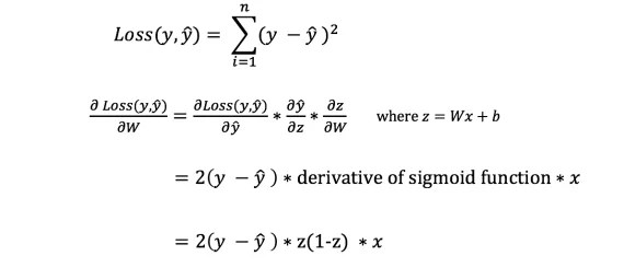
Phew! This was cumbersome, but it allowed us to get what we needed — the derivative (slope) of the loss function with respect to the weights. Now we can adjust the weights accordingly.

Let's add the backpropagation function to our Python code:

Checking the operation of the neural network

Now that we have our full code in Python to perform forward and back propagation, let's look at our neural network as an example and see how it works.

Ideal set of scales

Our neural network must learn the ideal set of weights to represent this function.

Let's train the neural network for 1500 iterations and see what happens. Looking at the iteration loss plot below, we can clearly see that the loss monotonically decreases to a minimum. This is consistent with the gradient descent algorithm we discussed earlier.

Let's look at the final prediction (output) from the neural network after 1500 iterations.

We did it! Our forward and backpropagation algorithm has shown that the neural network performs successfully, and the predictions converge on the true values.

Note that there is a slight difference between the predictions and the actual values. This is desirable because it prevents overfitting and allows the neural network to generalize better to unseen data.

Final Thoughts

I learned a lot in the process of writing my own neural network from scratch. Although libraries deep learning, such as TensorFlow and Keras, allow the creation deep networks without full understanding internal work neural network, I find it useful for aspiring Data Scientists to gain a deeper understanding of them.

I invested a lot of my personal time in this work, and I hope you find it useful!