Perspective matrices in the graphics API or the devil is in the details. Programming with DirectX9: Rotating Objects

Axonometry is a parallel projection. Table 3.3 first lists the matrices of orthographic projections onto coordinate planes obtained from their definitions.

Table 3.3.Matrixes of design transformations and projection

Orthographic projection on XOY		Orthographic projection on YOZ

Orthographic projection on XOZ		Orthographic projection onto the x=p plane

Trimetric transformation matrix to the XOY plane

Isometric transformation matrix to the XOY plane

Isometric projection matrix on the XOY plane

Oblique projection matrix on XOY	Free projection matrix on XOY

Cabinet projection matrix on XOY	Perspective transformation matrix with one vanishing point (the picture plane is perpendicular to the x-axis)

Perspective transformation matrix with one vanishing point (the picture plane is perpendicular to the y-axis)		Perspective transformation matrix with one vanishing point (the picture plane is perpendicular to the applicate axis)

Perspective transformation matrix with two vanishing points (the picture plane is parallel to the y-axis)		Perspective transformation matrix with three vanishing points (picture plane of arbitrary position)

Isometry, dimetry and trimetry are obtained by a combination of rotations followed by a projection from infinity. If you need to describe the projection onto the XOY plane, then you first need to carry out a rotation transformation by an angle relative to the ordinate axis, then to the angle relative to the abscissa axis. Table 3.3 shows the trimetric transformation matrix. To obtain a dimetric transformation matrix in which, for example, the distortion coefficients along the abscissa and ordinate axes will be equal, the relationship between the rotation angles must obey the relationship

That is, by choosing the angle , you can calculate the angle and determine the dimetric projection matrix. For an isometric transformation, the relationship between these angles turns into strictly defined values, which are:

Table 3.3 shows the isometric transformation matrix, as well as the isometric projection matrix onto the XOY plane. The need for matrices of the first type lies in their use in algorithms for removing invisible elements.

In oblique projections, the projecting straight lines form an angle with the projection plane that is different from 90 degrees. Table 3.3 shows the general matrix of oblique projection onto the XOY plane, as well as matrices of free and cabinet projections, in which:

Perspective projections (Table 3.3) are also represented by perspective transformations and perspective projections on the XOY plane. V X, V Y and V Z are projection centers - points on the corresponding axes. –V X, -V Y, -V Z will be the points at which bundles of straight lines parallel to the corresponding axes converge.

The observer's coordinate system is left coordinate system (Fig. 3.3), in which the z e axis is directed from the point of view forward, the x e axis is directed to the right, and the y e axis is directed upward. This rule is adopted to ensure that the x e and y e axes coincide with the x s and y s axes on the screen. Determining the values of the screen coordinates x s and y s for point P leads to the need to divide by the z e coordinate. To construct an accurate perspective image, it is necessary to divide by the depth coordinate of each point.

Table 3.4 shows the values of the vertex descriptor S(X,Y,Z) of the model (Fig. 2.1) subjected to rotation transformations and isometric transformation.

Table 3.4.Model vertex descriptors

Original model				M(R(z,90))xM(R(y,90))

The engine does not move the ship. The ship remains in place, and the engine moves the universe relative to it.

This is very an important part lessons, make sure you read it several times and understand it well.

Homogeneous coordinates

Until now, we have treated 3-dimensional vertices as (x, y, z) triplets. Let's introduce another parameter w and operate with vectors of the form (x, y, z, w).

Remember forever that:

If w == 1, then the vector (x, y, z, 1) is a position in space.
If w == 0, then the vector (x, y, z, 0) is the direction.

What does this give us? Ok, for rotation this does not change anything, since both in the case of rotating the point and in the case of rotating the direction vector you get the same result. However, there is a difference in the case of transfer. Translating the direction vector will give the same vector. We'll talk more about this later.

Homogeneous coordinates allow us, using one mathematical formula operate with vectors in both cases.

Transformation matrices

Introduction to Matrices

The easiest way to imagine a matrix is as an array of numbers, with a strictly defined number of rows and columns. For example, a 2x3 matrix looks like this:

However, in 3D graphics we will only use 4x4 matrices which will allow us to transform our vertices (x, y, z, w). The transformed vertex is the result of multiplying the matrix by the vertex itself:

Matrix x Vertex (in that order!!) = Transform. vertex

Quite simple. We'll be using this quite often, so it makes sense to have the computer do it:

In C++, using GLM:

glm::mat4 myMatrix; glm::vec4 myVector;

glm::

// Pay attention to the order! He is important! In GLSL: mat4 myMatrix ; vec4 myVector ;

// Don't forget to fill the matrix and vector with the necessary values here

vec4 transformedVector = myMatrix * myVector ;

// Yes, it's very similar to GLM :)

Try experimenting with these snippets.

Transfer Matrix

The transfer matrix looks like this:

where X, Y, Z are the values we want to add to our vector.

So, if we want to move the vector (10, 10, 10, 1) by 10 units in the X direction, we get:

... we get (20, 10, 10, 1) a homogeneous vector! Remember that the 1 in the w parameter means position, not direction, and our transformation did not change the fact that we are working with position.

Now let's see what happens if the vector (0, 0, -1, 0) represents a direction:

... and we get our original vector (0, 0, -1, 0). As was said earlier, a vector with parameter w = 0 cannot be transferred. Now is the time to put it into code. In C++, with GLM:

glm::

#include

// after

glm::mat4 myMatrix = glm::translate(glm::mat4(), glm::vec3(10.0 f, 0.0 f, 0.0 f));

glm::vec4 myVector(10.0 f, 10.0 f, 10.0 f, 0.0 f);

glm::vec4 transformedVector = myMatrix * myVector ;

vec4 transformedVector = myMatrix * myVector ;

In fact, you will never do this in a shader, most often you will do glm::translate() in C++ to calculate the matrix, pass it to GLSL, and then perform the multiplication in the shader

Identity matrix

This is a special matrix that doesn't do anything, but we're touching on it because it's important to remember that A times 1.0 equals A:

In C++: glm::mat4 myIdentityMatrix = glm::mat4(1.0 f); scaling matrices with a scale factor equal to 1 on all axes. Also, the identity matrix is a special case of the transfer matrix, where (X, Y, Z) = (0, 0, 0), respectively.

glm::vec4 transformedVector = myMatrix * myVector ;

// add #include and #include glm::mat4 myScalingMatrix = glm::scale(2.0 f, 2.0 f, 2.0 f);

Rotation matrix

More complicated than those discussed earlier. We'll omit the details here since you don't need to know this exactly for daily use. To get more detailed information you can follow the link Matrices and Quaternions FAQ (quite a popular resource and your language may be available there)

glm::vec4 transformedVector = myMatrix * myVector ;

// add #include and #include glm::vec3 myRotationAxis ( ?? , ?? , ?? );

glm::rotate(angle_in_degrees, myRotationAxis);

Putting transformations together So now we can rotate, translate and scale our vectors. Next step

It would be nice to combine transformations, which is implemented using the following formula:

TransformedVector = TranslationMatrix * RotationMatrix * ScaleMatrix * OriginalVector ;

ATTENTION! This formula actually shows that scaling is done first, then rotation is done, and only lastly is translation done. This is exactly how matrix multiplication works.

Be sure to remember what order all this is done in, because the order is really important, after all, you can check it yourself:
Take a step forward and turn left

Turn left and take a step forward

The difference is really important to understand because you will encounter this all the time. For example, when you work with game characters or some objects, always scale first, then rotate, and only then translate.

In fact, the above order is what you generally need for game characters and other items: scale it first if necessary; then you set its direction and then move it. For example, for a ship model (rotations removed for simplicity):
- Wrong Way:
- You move the ship to (10, 0, 0). Its center is now 10 units from the origin.
You scale your ship by 2 times. Each coordinate is multiplied by 2 “relative to the original”, which is far... So, you end up in a large ship, but its center is 2 * 10 = 20. Not what you wanted.
- The right way:
- You scale your ship by 2 times. You get a large ship, centered at the origin.

Now let's see what happens if the vector (0, 0, -1, 0) represents a direction:

glm::mat4 myModelMatrix = myTranslationMatrix * myRotationMatrix * myScaleMatrix ;

glm::

glm::vec4 myTransformedVector = myModelMatrix * myOriginalVector;

mat4 transform = mat2 * mat1 ;

vec4 out_vec = transform * in_vec ;

World, view and projection matrices For the rest of this tutorial, we'll assume we know how to render Blender's favorite 3D model, Suzanne the Monkey. World, view and projection matrices are

handy tool

to separate transformations.

World matrix

This model, just like our red triangle, is defined by a set of vertices, the coordinates of which are given relative to the center of the object, i.e. the vertex with coordinates (0, 0, 0) will be in the center of the object. Next we would like to move our model as the player controls it using the keyboard and mouse. All we do is apply scaling, then rotate and translate. These actions are performed for each vertex, in each frame (performed in GLSL, not C++!) and thereby our model moves on the screen.

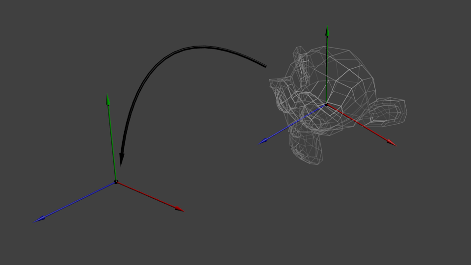
Now our peaks in world space. This is shown by the black arrow in the figure.

We have moved from object space (all vertices are defined relative to the center of the object) to world space (all vertices are defined relative to the center of the world).

This is shown schematically like this:

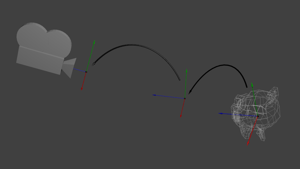
View matrix

To quote Futurama again: The engine does not move the ship. The ship remains in the same place, and the engine moves the universe around it. Try to imagine this in relation to a camera. For example, if you want to take a photograph of a mountain, you don't move the camera, you move the mountain. This is not possible in

real life

, but it's incredibly simple in computer graphics. and #include So, initially your camera is at the center of the world coordinate system. To move the world you need to enter another matrix. Let's say you want to move the camera 3 units to the RIGHT (+X), which is the equivalent of moving the entire world 3 units to the LEFT (-X). In code it looks like this:

// Add #include

glm::mat4 ViewMatrix = glm::translate(glm::mat4(), glm::vec3(-3.0 f, 0.0 f, 0.0 f));

glm::mat4 CameraMatrix = glm::LookAt(cameraPosition, // Camera position in world space cameraTarget // Indicates where you are looking in world space upVector // A vector indicating the upward direction. Typically (0, 1, 0));

And here is a diagram that shows what we do:

However, this is not the end.

Projection matrix

So now we're in camera space. This means that a vertex that receives coordinates x == 0 and y == 0 will be displayed in the center of the screen. However, when displaying an object, the distance to the camera (z) also plays a huge role. For two vertices with the same x and y, the vertex with a larger z value will appear closer than the other.

This is called perspective projection:

And luckily for us, a 4x4 matrix can do this projection:

// Creates a really hard to read matrix, but it's still a standard 4x4 matrix glm::mat4 projectionMatrix = glm::perspective (glm::radians (FoV), // Vertical field of view in radians. Typically between 90° (very wide) and 30° (narrow) 4.0 f/3.0 f, // Aspect ratio. Depends on the size of your window. Note that 4/3 == 800/600 == 1280/960 0.1 f // Near clipping plane. Must be greater than 0. 100.0f // Far clipping plane.);

We have moved from Camera Space (all vertices are defined relative to the camera) to Homogeneous Space (all vertices are in a small cube. Everything that is inside the cube is displayed on the screen).

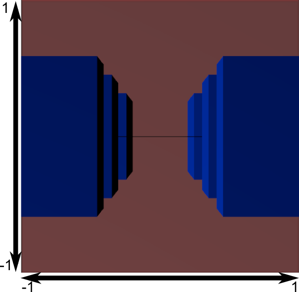
Now let's look at following images, so that you can better understand what is happening with the projection. Before projection, we have blue objects in camera space, while the red figure shows the camera view, i.e. everything that the camera sees.

Using the Projection Matrix gives the following effect:

In this image, the camera view is a cube and all objects are deformed. Objects that are closer to the camera appear large, and those that are further away appear small. Just like in reality!

This is what it will look like:

The image is square, so the following mathematical transformations are applied to stretch the image according to current sizes window:

And this image is what will actually be output.

Combining transformations: ModelViewProjection matrix

... Just the standard matrix transformations you already love!

// C++ : matrix calculation glm::mat4 MVPmatrix = projection * view * model ; // Remember! IN reverse order!

// GLSL: Apply Matrix transformed_vertex = MVP * in_vertex ;

Putting it all together

The first step is creating our MVP matrix. This must be done for each model you display.

// Throw matrix: 45° field of view, 4:3 aspect ratio, range: 0.1 unit<->100 units glm::mat4 Projection = glm::perspective(glm::radians(45.0 f), 4.0 f / 3.0 f, 0.1 f, 100.0 f); // Or, for the orthocamera glm::mat4 View = glm::lookAt(glm::vec3(4, 3, 3), // Camera is in world coordinates (4,3,3) glm::vec3(0, 0, 0), // And directed to the origin glm::vec3(0, 1, 0) // "Head" is on top); // Model matrix: identity matrix (The model is at the origin) glm::mat4 Model = glm::mat4(1.0 f); // Individually for each model // The final ModelViewProjection matrix, which is the result of multiplying our three matrices glm::mat4 MVP = Projection * View * Model ; // Remember that matrix multiplication is done in reverse order

The second step is to pass this to GLSL:

// Get the variable handle in the shader // Only once during initialization. GLuint MatrixID = glGetUniformLocation(programID, "MVP"); // Pass our transformations to the current shader // This is done in the main loop, since each model will have a different MVP matrix (at least part M) glUniformMatrix4fv(MatrixID, 1, GL_FALSE, &MVP[0][0]);

The third step is to use the received data in GLSL to transform our vertices.

// Vertex input data, different for all executions of this shader. layout (location = 0 ) in vec3 vertexPosition_modelspace ; // Values that remain constant for the entire mesh. uniform mat4 MVP ; void main ()(// Output position of our vertex: MVP * position

gl_Position = MVP * vec4(vertexPosition_modelspace, 1);

)

Ready! Now we have the same triangle as in Lesson 2, still located at the origin (0, 0, 0), but now we see it in perspective from the point (4, 3, 3).

In Lesson 6, you'll learn how to change these values dynamically using your keyboard and mouse to create the camera you're used to seeing in games. But first, we'll learn how to give our models colors (Lesson 4) and textures (Lesson 5).
Tasks
Modify ModelMatrix to move, rotate and scale triangle
Use the previous task, but with in different order operations. Pay attention to the result.

At some point, any developer in the field computer graphics The question arises: how do these promising matrices work? Sometimes the answer is very difficult to find and, as usually happens, the majority of developers give up halfway through the task.

This is not a solution to the problem! Let's figure it out together!

Let's be realistic with a practical bias and take as a test subject OpenGL versions 3.3. Starting from this version, each developer is required to independently implement the module matrix operations. Great, this is what we need. Let us decompose our difficult task and highlight the main points. Some facts from the OpenGL specification:

Matrices are stored in columns (column-major);
Homogeneous coordinates;
Canonical clipping volume (CVV) in a left-handed coordinate system.

There are two ways to store matrices: column-major and row-major. In lectures on linear algebra, the row-major scheme is used. By by and large The representation of matrices in memory does not matter, because a matrix can always be converted from one representation to another by simple transposition. And since there is no difference, then for all subsequent calculations we will use classic row-major matrices. When programming OpenGL there is little trick, which allows you to refuse to transpose matrices while maintaining classic row-major calculations. The matrix must be transferred to the shader program as is, and in the shader the multiplication should be carried out not between a vector and a matrix, but between a matrix and a vector.

Homogeneous coordinates are not a very tricky system with a number of simple rules on converting conventional Cartesian coordinates into homogeneous coordinates and vice versa. A homogeneous coordinate is a row matrix of dimension . In order to convert a Cartesian coordinate into a homogeneous coordinate, it is necessary x, y And z multiply by any real number w(except 0). Next, you need to write the result in the first three components, and the last component will be equal to the multiplier w. In other words:
- Cartesian coordinates
w– real number not equal to 0

- homogeneous coordinates

A little trick: If w equals one, then all that is needed for translation is to transfer the components x, y And z and assign one to the last component. That is, get a row matrix:

A few words about zero quality w. From the point of view of homogeneous coordinates, this is quite acceptable. Homogeneous coordinates allow you to distinguish between points and vectors. In a Cartesian coordinate system, such a division is impossible.

- point where ( x, y, z) – Cartesian coordinates

- vector, where ( x, y, z) – radius vector

The reverse translation of a vertex from homogeneous coordinates to Cartesian coordinates is carried out as follows. All components of a row matrix must be divided by the last component. In other words:

- homogeneous coordinates
- Cartesian coordinates

The main thing you need to know is that all OpenGL clipping and rasterization algorithms work in Cartesian coordinates, but before that all transformations are performed in homogeneous coordinates. The transition from homogeneous coordinates to Cartesian coordinates is carried out in hardware.

Canonical clipping volume (CVV) is one of the least documented parts of OpenGL. As can be seen from Fig. 1 CVV is an axis-aligned cube centered at the origin and with an edge length equal to two. Everything that falls within the CVV area is subject to rasterization, everything that is outside the CVV is ignored. Anything that partially falls outside the CVV is subject to pruning algorithms. The most important thing you need to know is that the CVV coordinate system is left-handed!

Rice. 1. Canonical OpenGL clipping volume (CVV)

Left-handed coordinate system? How can this be, since the specification for OpenGL 1.0 clearly states that the coordinate system used is right-handed? Let's figure it out.

Rice. 2. Coordinate systems

As can be seen from Fig. The 2 coordinate systems differ only in the direction of the axis Z. OpenGL 1.0 actually uses right-handed user system coordinates But the CVV coordinate system and the user coordinate system are two completely different things. Moreover, as of version 3.3, there is no longer such a thing as standard system OpenGL coordinates. As mentioned earlier, the programmer himself implements the matrix operations module. Formation of rotation matrices, formation of projection matrices, search for an inverse matrix, matrix multiplication are minimum set operations included in the matrix operations module. Two logical questions arise. If the visibility volume is a cube with an edge length equal to two, then why is a scene several thousand in size visible on the screen? At what point does the user coordinate system convert to the CVV coordinate system? Projection matrices are precisely the entity that deals with these issues.

The main idea of the above is that the developer himself is free to choose the type of user coordinate system and must correctly describe the projection matrices. This completes the facts about OpenGL and it’s time to put everything together.

One of the most common and difficult to comprehend matrices is the perspective transformation matrix. So how does it relate to CVV and the user coordinate system? Why do objects become smaller as their distance from the observer increases? To understand why objects shrink as distance increases, let's look at the matrix transformations of a 3D model step by step. It's no secret that any three-dimensional model consists of a finite list of vertices that undergo matrix transformations completely independently of each other. In order to determine the coordinate of a three-dimensional vertex on a two-dimensional monitor screen, you need to:

Convert Cartesian coordinate to homogeneous coordinate;
Multiply the homogeneous coordinate by the model matrix;
The result is multiplied by the view matrix;
Multiply the result by the projection matrix;
Convert the result from homogeneous coordinates to Cartesian coordinates.

The conversion of Cartesian coordinates to homogeneous coordinates was discussed earlier. The geometric meaning of the model matrix is to translate the model from local system coordinates in global system coordinates Or, as they say, move the vertices out of the model space into the world space. Let's put it simply, a three-dimensional object loaded from a file is located in model space, where coordinates are measured relative to the object itself. Next, using the model matrix, the model is positioned, scaled and rotated. As a result, all vertices of the 3D model receive actual homogeneous coordinates in the 3D scene. Model space relative to world space is local. From the model space, coordinates are transferred to world space (from local to global). For this purpose, a model matrix is used.

Now let's move on to step three. This is where the view space comes into play. In this space, coordinates are measured relative to the position and orientation of the observer as if he were the center of the world. The view space is local relative to the world space, so the coordinates must be entered into it (and not taken out, as in the previous case). Direct matrix transformation removes coordinates from some space. In order to introduce them into it, on the contrary, it is necessary to invert the matrix transformation, therefore the type transformation is described by the inverse matrix. How to get this inverse matrix? First, let's get the direct observer matrix. What characterizes an observer? The observer is described by the coordinate in which he is located and the viewing direction vectors. The observer always looks in the direction of his local axis Z. The observer can move around the scene and make turns. In many ways, this resembles the meaning of the model matrix. By and large, this is how it is. However, for an observer, the scaling operation is meaningless, therefore, an equal sign cannot be put between the model matrix of the observer and the model matrix of a three-dimensional object. The model matrix of the observer is the desired direct matrix. By inverting this matrix, we obtain the view matrix. In practice, this means that all vertices in global homogeneous coordinates will receive new homogeneous coordinates relative to the observer. Accordingly, if the observer saw a certain vertex, then the value of the homogeneous coordinate z of a given vertex in view space will definitely be a positive number. If the vertex was behind the observer, then the value of its homogeneous coordinate z in view space will definitely be a negative number.

Step four is the most interesting step. Previous steps were discussed in such detail intentionally so that the reader has a complete picture of all the operands of the fourth step. At the fourth step, homogeneous coordinates are transferred from the view space to the CVV space. Once again, the fact is emphasized that all potentially visible vertices will have a positive value of the homogeneous coordinate z.

Consider a matrix of the form:

And a point in the observer’s homogeneous space:

Let's multiply the homogeneous coordinate by the matrix in question:

Let's convert the resulting homogeneous coordinates into Cartesian coordinates:

Let's say there are two points in view space with the same coordinates x And y, but with different coordinates z. In other words, one of the points is behind the other. Due to perspective distortion, the observer must see both points. Indeed, it is clear from the formula that due to division by the coordinate z, compression occurs to the origin point. How more value z(the further the point is from the observer), the stronger the compression. This is the explanation for the perspective effect.

The OpenGL specification states that clipping and rasterization operations are performed in Cartesian coordinates, and the process of converting homogeneous coordinates to Cartesian coordinates is performed automatically.

Matrix (1) is a template for a perspective projection matrix. As mentioned earlier, the task of the projection matrix consists of two points: setting a user coordinate system (left-handed or right-handed), transferring the observer's visibility volume to CVV. Let's derive a perspective matrix for a left-handed user coordinate system.

The projection matrix can be described using four parameters (Fig. 3):

Viewing angle in radians ( fovy);
Aspect Ratio ( aspect);
Distance to the nearest clipping plane ( n);
Distance to the far clipping plane ( f).

Rice. 3. Perspective volume of visibility

Let's consider the projection of a point in the observer's space onto the front edge of the cutoff of the perspective volume of visibility. For greater clarity, in Fig. 4 shows a side view. It should also be taken into account that the user coordinate system coincides with the CVV coordinate system, that is, the left-handed coordinate system is used everywhere.

Rice. 4. Projecting an arbitrary point

Based on the properties of similar triangles, the following equalities are true:

Let's express yꞌ and xꞌ:

In principle, expressions (2) are sufficient to obtain the coordinates of the projection points. However, to properly screen three-dimensional objects, you need to know the depth of each fragment. In other words, it is necessary to store the value of the component z. This is the value used for OpenGL depth tests. In Fig. 3 it is clear that the value zꞌ is not suitable as a fragment depth, because all point projections can same value zꞌ. The way out of this situation is to use the so-called pseudo-depth.

Pseudo-depth properties:

Pseudo-depth is calculated based on the value z;
The closer the point is to the observer, the less value the pseudodepth has;
All points lying on the front plane of the visibility volume have a pseudo-depth value of -1;
All points lying on the far cutting plane of the visibility volume have a pseudo-depth value of 1;
All fragments lying inside the visibility volume have a pseudo-depth value in the range [-1 1].

Let's derive the formula by which pseudo-depth will be calculated. Let's take the following expression as a basis:

Odds a And b needs to be calculated. In order to do this, we use the properties of pseudo-depths 3 and 4. We obtain a system of two equations with two unknowns:

Let's add both parts of the system and multiply the result by the product fn, wherein f And n cannot be equal to zero. We get:

Let's open the brackets and rearrange the terms so that only the part with A, and on the right only with b:

Let's substitute (6) into (5). Let's convert the expression to a simple fraction:

Multiply both sides by -2fn, wherein f And n cannot be equal to zero. Let us present similar ones, rearrange the terms and express b:

Let's substitute (7) into (6) and express a:

Accordingly the components a And b are equal:

Now let’s substitute the obtained coefficients into the workpiece matrix (1) and see what happens to the coordinate z for an arbitrary point in the observer's homogeneous space. The substitution is performed as follows:

Let the distance to the front cutting plane n is equal to 2, and the distance to the far clipping plane f equals 10. Consider five points in the observer’s homogeneous space:

Mutual arrangement points and volume of visibility

Dot	Meaning	Description
1	1	The point is located in front of the front cutting plane of the visibility volume. Doesn't pass rasterization.
2	2	The point is located on the front edge of the visibility volume cutoff. Undergoing rasterization.
3	5	The point is located between the front clipping edge and the far clipping edge of the visibility volume. Undergoing rasterization.
4	10	The point is located on the far edge of the visibility volume cutoff. Undergoing rasterization.
5	20	The point is located beyond the far edge of the visibility volume cutoff. Does not pass rasterization.

Let's multiply all points by matrix (8), and then convert the resulting homogeneous coordinates to Cartesian coordinates . To do this, we need to calculate the values of new homogeneous components And .
Point 1:

Note that the homogeneous coordinate absolutely correctly positioned in CVV, and most importantly, the OpenGL depth test is now possible, because pseudo-depth fully satisfies the test requirements.

With coordinate z We figured it out, let's move on to the coordinates x And y. As mentioned earlier, the entire perspective volume of visibility must fit into the CVV. The length of the CVV edge is two. Accordingly, the height and width of the perspective volume of visibility must be compressed to two conventional units.

We have at our disposal a corner fovy and magnitude aspect. Let's express height and width using these values.

Rice. 5. Visibility volume

From Fig. 5 it is clear that:

Now you can get final look perspective projection matrix for a custom left-handed coordinate system working with CVV OpenGL:

This completes the derivation of matrices.

A few words about DirectX - the main competitor of OpenGL. DirectX differs from OpenGL only in the dimensions of the CVV and its positioning. In DirectX, a CVV is a rectangular parallelepiped with lengths along its axes x And y equal to two, and along the axis z length is equal to one. Range x And y is [-1 1], and the range z equal to . As for the CVV coordinate system, DirectX, like OpenGL, uses a left-handed coordinate system.

To display perspective matrices for a custom right-handed coordinate system, you need to redraw Fig. 2, Fig. 3 and Fig. 4 taking into account the new axis direction Z. Further calculations are completely similar, up to the sign. For DirectX matrices, pseudo-depth properties 3 and 4 are modified to suit the range.

At this point, the topic of promising matrices can be considered closed.

To describe in detail the methods for point feature tracking, camera calibration, and 3D object reconstruction, it is necessary to introduce a perspective design model and describe the geometric properties of this transformation. The points of several images obtained using perspective projection have special relationships with each other, which are described by epipolar geometry. The models of these relationships must be examined in detail, because Almost all three-dimensional reconstruction methods require the evaluation of corresponding models and rely on their properties.

It is necessary to separately note the assumption that all source images capture the same scene, i.e. each image is a view of the scene from a specific camera. Therefore, for convenience of description, the concept of a view is introduced, as an image with an associated camera model from which it was obtained.

Perspective projection

The perspective projection model corresponds to an ideal pinhole camera. This model quite closely matches the image construction process in most modern photo and video cameras. However, due to the limitations of modern optics, the actual process is somewhat different from the pinhole camera model. Differences between the real process and the model are called distortions and are modeled separately.

The model of the simplest pinhole camera is convenient in that it is completely described by the center of projection and the position of the image plane. Therefore, the projection of any scene point in the image can be found as the intersection of the ray connecting the center of the projection and the scene point with the image plane.

The simplest model of perspective projection

Let's consider the simplest case when the center of the camera projection (focus) is placed at the origin of the coordinate system, and the image plane coincides with the Z=1 plane. Let (X,Y,Z) be the coordinates of a point in 3-dimensional space, and (x,y) be the projection of this point onto image I. The perspective projection in this case is described by the following equations:

In matrix form using homogeneous coordinates, these equations are rewritten as follows:

(2.2)

The plane located at a distance of 1 from the center of the projection and perpendicular to the optical axis is called the ideal image plane. The optical axis intersects the ideal image plane at a point c, called the principal point. An illustration of the simplest case of perspective projection is shown in Fig. 1.

Internal camera calibration

The simplest case of perspective projection almost always does not correspond to the real camera. The distance from the projection center to the image plane, i.e. the focal length, denoted by f, is usually not equal to 1. Also, the coordinates of a point in the image plane may not coincide with absolute coordinates. Using digital camera, the relationship between the coordinates of a point in the image and the absolute coordinates of a point on an ideal plane, is determined by the shape and size of the pixels of the matrix.

Let us denote the pixel dimensions of a digital camera matrix as p x , p y , the pixel inclination angle as α , and the principal point as , Fig. 2. Then the coordinates of the point (x,y) in the image corresponding to the point (x R , y R) on the ideal plane are determined by the expression:

(2.3)

If f x ,f y is the focal length f, measured in pixel widths and heights, and tan(α)*f/p y is denoted as s, then formula 2.3 is transformed into:

(2.4)

The K matrix is called the camera's internal calibration matrix. In most cases, in real digital cameras the pixel angle is close to straight, i.e. parameter s=0, and the width and height of the pixel are equal. The principle point is usually located in the center of the image. Therefore, matrix K can be written as:

(2.5)

This assumption about the form of the K matrix is widely used to simplify algorithms for determining camera internal calibration, as well as in synthetic image modeling needed to evaluate the quality and efficiency of 3D reconstruction methods.

External camera calibration

Let M be a scene point in 3-dimensional space. Any movement is a Euclidean transformation of space, therefore in homogeneous coordinates it is expressed as:

(2.6)

where R is the rotation matrix, T= T is the translation vector.

The movement of the camera relative to the scene is equivalent to the reverse movement of the points of the scene relative to the camera, therefore it is equal to:

(2.7)

where R, T is the rotation matrix and the camera movement vector relative to the scene. Matrix C is called matrix external calibration cameras. The matrix C -1 is called the matrix camera movements. Thus, the external camera calibration matrix translates the coordinates of the scene points from the scene coordinate system to the coordinate system associated with the camera.

Complete Perspective Projection Model

From expressions 2.1, 2.4, 2.7, we can derive an expression for an arbitrary perspective projection for any camera with an arbitrary orientation and position in space:

In a more concise form, taking into account the previous notation, this formula can be written as:

The matrix P is called the camera projection matrix.

By analogy with the general perspective transformation, let us first consider the simplest case of a perspective transformation of a plane. Let the plane p coincide with the plane Z=0, then the homogeneous three-dimensional coordinates of any of its points are M=. For any camera with a projection matrix P, the perspective transformation of the plane is described by a 3*3 matrix:

Since any plane in 3-dimensional space can be transferred to the Z = 0 plane by the Euclidean transformation of rotation and translation, which is equivalent to multiplying the camera matrix P by the transformation matrix L, then the perspective display of an arbitrary plane in space is described by linear transformation with a 3*3 matrix.

Perspective plane transformation is also called homography. In matrix form, the perspective transformation of the plane is written as m=HM.

Geometry of two images

The scene captured on all source images is considered motionless, therefore the relative position of the projections of the scene points on different frames cannot change randomly. The restrictions imposed on the location of point projections obviously depend on the parameters of the cameras and their position relative to each other. Therefore, determining models of such restrictions provides some information about the relative positions of the cameras from which the images were obtained.

Perspective plane transformation

If the centers of the two cameras coincide, then the points on the image planes of both cameras are translated into each other by a perspective transformation of the plane. In this case, the transformation of points between images does not depend on the shape of the 3-dimensional scene, but depends only on the relative position of the image planes.

If the entire scene or part of it is a plane, then its images on different types with non-coinciding camera centers can be converted into each other by a homography transformation. Let p be the observed plane, H 1 be the homography transformation between plane p and the image I 1, H 2 - homography transformation between plane p and image I 2. Then the homography transformation H 12 between images I 1 And I 2 can be output as follows:

H 12 does not depend on the parameterization of the plane p, and therefore does not depend on the coordinate system in space

Most methods for determining the coordinates of 3D points from their projections and methods for reconstructing a 3D scene are based on the assumption that the camera center moves between views. Therefore, if the centers of cameras of several types coincide, these methods will give incorrect results. Such camera configurations must be detected and handled in a special way.

Since the homography transformation is written in homogeneous coordinates, the matrix H is defined up to scale. It has 8 degrees of freedom, and is parameterized by 8 variables. Every known pair of corresponding points m 1 And m 2 in the first and second image respectively gives 2 linear equations from the elements of the matrix H. Therefore, 4 known pairs of corresponding points are sufficient to compose a system of linear equations of 8 equations with 8 unknowns. According to this system, the homography H can be uniquely determined if no three of the points lie on the same line.

Fundamental Matrix

Let's consider the case when the centers of the two types of cameras do not coincide. Let C 1 And C 2- centers of two cameras, M - 3-dimensional point of the scene, m 1 And m 2- projections of point M onto the first and second images, respectively. Let P be a plane passing through the point M and the centers of the cameras C 1 And C 2. Plane P intersects the image planes of the first and second views along straight lines l 1 And l 2. Since the rays C 1 M And C 2 M lie in the plane P, then it is obvious that the points m 1 And m 2 lie on straight lines l 1 And l 2 respectively. You can give more general statement that the projections of any point M" lying in the plane P onto both images must lie on straight lines l 1 And l 2. These lines are called epipolar lines. The plane P is called the epipolar plane.

Two views of the same scene are called a stereo pair, and a segment C 1 C 2, connecting the centers of the cameras is called the base of the stereo pair (baseline) or stereo base. Any epipolar plane passes through the segment C 1 C 2. Let C 1 C 2 intersects the first and second images at points e 1 And e 2 respectively. Points e 1 And e 2 are called epipolar points or epipoles. All epipolar lines intersect at points e 1 And e 2 in the first and second image respectively. The set of epipolar planes is a beam intersecting along the stereo base C 1 C 2. The many epipolar lines in both images also represent bundles of straight lines intersecting at e 1 And e 2 .

Points m 1 And m 2 are called corresponding if they are projections of the same scene point M. Epipolar lines l 1 And l 2 are called corresponding if they lie in the same epipolar plane P. If the epipolar plane P passes through a point m 1, then the epipolar lines l 1 And l 2, lying in it are called corresponding to the point m 1.

Restriction on the position of the corresponding points m 1 And m 2, which follows from epipolar geometry, can be formulated as follows: point m 2, corresponding m 1, must lie on the epipolar line l 2, corresponding m 1. This condition is called the epipolar constraint. In homogeneous coordinates, the condition that a point m lies on the line l written as l T m=0. The epipolar line also passes through the epipolar point. Equation of a line passing through points m 1 And e 1 can be written as:

l 1 ∼ x m 1,

Where x- an antisymmetric matrix of dimension 3*3 such that, x m 1- vector product m 1 And e 1.

For the corresponding epipolar lines l 1 And l 2 right:

Where P+- pseudoinversion of matrix P.

The matrix F is called the fundamental matrix. It is a linear operator that associates each point m 1 its corresponding epipolar line l 2. For each pair of corresponding points m 1 And m 2 right

m T 2 Fm 1 =0

This is a formulation of the epipolar constraint through the fundamental matrix.

The fundamental matrix has 7 degrees of freedom. Each pair of corresponding points m 1 And m 2 defines one linear equation for the elements of the matrix, so it can be calculated from the known 7 pairs of corresponding points.

The epipolar constraint is valid for any pairs of corresponding points located on ideal planes of two types. If the internal calibration matrices are known K 1 And K2 cameras of both types, then the epipolar constraint for the corresponding points on ideal planes is written as:

The matrix E is called significant matrix. It can be shown that the essential matrix can also be obtained from the relative positions of the cameras.

Let P 1 =(I|0) And P 2 =(R|-RT)- two design matrices with calibration K = I. Then the design equations for the ideal plane of both cameras are written in the form:

Let's find the epipolar line in the second view corresponding to the point m" 1 on the first. To do this, it is enough to project onto the second view two points lying on the ray (C 1 ,m" 1) to the second view, for example the center of the first camera (0,0,0,1) T and a point on the infinity plane (x" 1 ,y" 1 ,z" 1 ,0) T. The projections of these points will be -RT, and R(x" 1 ,y" 1 ,z" 1 ,0) T. Epipolar Line Equation l 2, passing through both of these points is given as a vector product:

l 2 =RT×R(x" 1 ,y" 1 ,z" 1) T =R(T×(x" 1 ,y" 1 ,z" 1) T)

In matrix form, a vector is not a product T×(x" 1 ,y" 1 ,z" 1) T can be written using the matrix S:

Then the epipolar constraint on points in the ideal plane is written as:

Expressing the essential matrix in terms of the external calibration parameters of the two cameras is used to calculate the relative positions of the cameras.

Geometric properties of three or more images

Let C 1,C 2 And C 3- centers of three views of the same three-dimensional scene. In this case, epipolar constraints are imposed on the corresponding points of any pair of species. If the projections of two points are known m 1 And m 2 to the first and second views, then the position of the projection to the third image can be found as the intersection of two epipolar views corresponding to the points m 1 And m 2.

According to two known projections m 1 And m 2 Using two images with a known calibration, the position of point M in space can be determined. Therefore, if the calibration of the third image is known, then the projection of point M onto the third view can be determined by a simple projection.

Constraints imposed on the position of corresponding points in more than two images can also be written in linear form. For three types, these restrictions are written in the form of a trifocal tensor, for four types - in the form of a quadrifocal tensor. However, computing these constraints is equivalent to calculating the gauge of all three or four views in projective space. These types of restrictions are not used in this work and therefore are not discussed in more detail.

At a certain point, any developer in the field of computer graphics has a question: how do these promising matrices work? Sometimes the answer is very difficult to find and, as usually happens, the majority of developers give up halfway through the task.

This is not a solution to the problem! Let's figure it out together!

Let's be realistic with a practical bias and take OpenGL version 3.3 as a test subject. Starting from this version, each developer is required to independently implement the matrix operations module. Great, this is what we need. Let us decompose our difficult task and highlight the main points. Some facts from the OpenGL specification:

Matrices are stored in columns (column-major);
Homogeneous coordinates;
Canonical clipping volume (CVV) in a left-handed coordinate system.

There are two ways to store matrices: column-major and row-major. In lectures on linear algebra, the row-major scheme is used. By and large, the representation of matrices in memory does not matter, because a matrix can always be converted from one type of representation to another by simple transposition. And since there is no difference, then for all subsequent calculations we will use classic row-major matrices. When programming OpenGL, there is a little trick that allows you to avoid transposing matrices while maintaining classic row-major calculations. The matrix must be transferred to the shader program as is, and in the shader the multiplication should be carried out not between a vector and a matrix, but between a matrix and a vector.

Homogeneous coordinates are not a very tricky system with a number of simple rules for converting familiar Cartesian coordinates into homogeneous coordinates and vice versa. A homogeneous coordinate is a row matrix of dimension . In order to convert a Cartesian coordinate into a homogeneous coordinate, it is necessary x, y And z multiply by any real number w(except 0). Next, you need to write the result in the first three components, and the last component will be equal to the multiplier w. In other words:
- Cartesian coordinates
w– real number not equal to 0

- homogeneous coordinates

A little trick: If w equals one, then all that is needed for translation is to transfer the components x, y And z and assign one to the last component. That is, get a row matrix:

Rice. 1. Canonical OpenGL clipping volume (CVV)

Left-handed coordinate system? How can this be, since the specification for OpenGL 1.0 clearly states that the coordinate system used is right-handed? Let's figure it out.

Rice. 2. Coordinate systems

As can be seen from Fig. The 2 coordinate systems differ only in the direction of the axis Z. OpenGL 1.0 does use a right-handed user coordinate system. But the CVV coordinate system and the user coordinate system are two completely different things. Moreover, as of version 3.3, there is no longer any such thing as a standard OpenGL coordinate system. As mentioned earlier, the programmer himself implements the matrix operations module. Formation of rotation matrices, formation of projection matrices, search for an inverse matrix, multiplication of matrices - this is the minimum set of operations included in the matrix operations module. Two logical questions arise. If the visibility volume is a cube with an edge length equal to two, then why is a scene several thousand in size visible on the screen? At what point does the user coordinate system convert to the CVV coordinate system? Projection matrices are precisely the entity that deals with these issues.

Convert Cartesian coordinate to homogeneous coordinate;
Multiply the homogeneous coordinate by the model matrix;
The result is multiplied by the view matrix;
Multiply the result by the projection matrix;
Convert the result from homogeneous coordinates to Cartesian coordinates.

The conversion of Cartesian coordinates to homogeneous coordinates was discussed earlier. The geometric meaning of the model matrix is to transfer the model from a local coordinate system to a global coordinate system. Or, as they say, move the vertices out of the model space into the world space. Let's put it simply, a three-dimensional object loaded from a file is located in model space, where coordinates are measured relative to the object itself. Next, using the model matrix, the model is positioned, scaled and rotated. As a result, all vertices of the 3D model receive actual homogeneous coordinates in the 3D scene. Model space relative to world space is local. From the model space, coordinates are transferred to world space (from local to global). For this purpose, a model matrix is used.

Step four is the most interesting step. The previous steps were discussed in such detail intentionally so that the reader has a complete picture of all the operands of the fourth step. At the fourth step, homogeneous coordinates are transferred from the view space to the CVV space. Once again, the fact is emphasized that all potentially visible vertices will have a positive value of the homogeneous coordinate z.

Consider a matrix of the form:

And a point in the observer’s homogeneous space:

Let's multiply the homogeneous coordinate by the matrix in question:

Let's convert the resulting homogeneous coordinates into Cartesian coordinates:

Let's say there are two points in view space with the same coordinates x And y, but with different coordinates z. In other words, one of the points is behind the other. Due to perspective distortion, the observer must see both points. Indeed, it is clear from the formula that due to division by the coordinate z, compression occurs to the origin point. The higher the value z(the further the point is from the observer), the stronger the compression. This is the explanation for the perspective effect.

The projection matrix can be described using four parameters (Fig. 3):

Viewing angle in radians ( fovy);
Aspect Ratio ( aspect);
Distance to the nearest clipping plane ( n);
Distance to the far clipping plane ( f).

Rice. 3. Perspective volume of visibility

Rice. 4. Projecting an arbitrary point

Based on the properties of similar triangles, the following equalities are true:

Let's express yꞌ and xꞌ:

In principle, expressions (2) are sufficient to obtain the coordinates of the projection points. However, to properly screen three-dimensional objects, you need to know the depth of each fragment. In other words, it is necessary to store the value of the component z. This is the value used for OpenGL depth tests. In Fig. 3 it is clear that the value zꞌ not suitable as a fragment depth, because all point projections have the same value zꞌ. The way out of this situation is to use the so-called pseudo-depth.

Pseudo-depth properties:

Pseudo-depth is calculated based on the value z;
The closer the point is to the observer, the less value the pseudodepth has;
All points lying on the front plane of the visibility volume have a pseudo-depth value of -1;
All points lying on the far cutting plane of the visibility volume have a pseudo-depth value of 1;
All fragments lying inside the visibility volume have a pseudo-depth value in the range [-1 1].

Let's derive the formula by which pseudo-depth will be calculated. Let's take the following expression as a basis:

Odds a And b needs to be calculated. In order to do this, we use the properties of pseudo-depths 3 and 4. We obtain a system of two equations with two unknowns:

Let's add both parts of the system and multiply the result by the product fn, wherein f And n cannot be equal to zero. We get:

Let's open the brackets and rearrange the terms so that only the part with A, and on the right only with b:

Let's substitute (6) into (5). Let's convert the expression to a simple fraction:

Multiply both sides by -2fn, wherein f And n cannot be equal to zero. Let us present similar ones, rearrange the terms and express b:

Let's substitute (7) into (6) and express a:

Accordingly the components a And b are equal:

Let the distance to the front cutting plane n is equal to 2, and the distance to the far clipping plane f equals 10. Consider five points in the observer’s homogeneous space:

The relative position of the point and volume of visibility

Dot	Meaning	Description
1	1	The point is located in front of the front cutting plane of the visibility volume. Doesn't pass rasterization.
2	2	The point is located on the front edge of the visibility volume cutoff. Undergoing rasterization.
3	5	The point is located between the front clipping edge and the far clipping edge of the visibility volume. Undergoing rasterization.
4	10	The point is located on the far edge of the visibility volume cutoff. Undergoing rasterization.
5	20	The point is located beyond the far edge of the visibility volume cutoff. Does not pass rasterization.

Note that the homogeneous coordinate absolutely correctly positioned in CVV, and most importantly, the OpenGL depth test is now possible, because pseudo-depth fully satisfies the test requirements.

We have at our disposal a corner fovy and magnitude aspect. Let's express height and width using these values.

Rice. 5. Visibility volume

From Fig. 5 it is clear that:

Now we can get the final view of the perspective projection matrix for a custom left-handed coordinate system working with CVV OpenGL:

This completes the derivation of matrices.

At this point, the topic of promising matrices can be considered closed.