Connecting cells in excel. The best alternative to the concatenate and merge text function in excel. Merging values ​​from cells

Previously, we have already considered the question “How to split one column of data into several in Excel 2007?” But what to do if you need to do the reverse operation? The question of how to combine (glue, concatenate) the contents of several cells in Excel 2007 will be discussed below.

Let's consider two ways.

The first way to combine cells in Excel 2007 is to use the “CONCATENATE” function (Text category). This function combines the contents of cells while allowing you to combine them with free text. As an example, consider an equation familiar to everyone from childhood))

In the Function Wizard window that opens, select the Text category and select the CONCATENATE function. Then click OK

In the next window, enter the arguments and click OK.

As a result we have))

This was the first way to combine the contents of multiple cells in Excel 2007. Let's look at another one below.

The second way to merge cells in Excel 2007 is to use the “&” gluing symbol.

To combine (glue) the contents of cells, the “&” symbol is used. This symbol must be placed at each cell connection point, just as the “+” symbol is placed when adding several numbers. If, in addition to gluing cells, you also need to add some character (dot, space, word), then this text must be enclosed in quotes. See below

Example of gluing without spaces

Example of gluing with spaces

I would like to draw your attention to the fact that the last example can be combined with the LEWSIM function and thus obtain a surname with initials.

All! Choose a method more convenient for you and use it! Have a nice work)

When designing tables to display information more clearly, it becomes necessary to combine several cells into one. This is often used, for example, when specifying one common data header that has different meanings. You can see an example of such information display in the image below. Read on to learn how to merge cells in Excel step by step. You can merge not only horizontally, it is possible to merge vertically, as well as groups of horizontal and vertical cells.

An example of combining a digit with one header “Digit” and different data

How to merge cells in excel

There are two ways to merge cells. The first is using the context menu through the format. Select all the cells that you want to merge and right-click on the selected area. In the drop-down context menu, select “Format Cells...”.

In the format window, go to the “Alignment” tab and in the display block, check the “merge cells” box.

Check the “merge cells” option in the “Alignment” tab

If there is any data in the cells, Excel issues a warning every time that all data except the top left one is lost. Therefore, be careful when merging and do not lose important data. If you still need to merge cells with data, click “OK” to agree.

In my case, out of 10 numbers in the cells in the merge area, only the number “1” from the top left cell remained.

By default, Excel aligns data to the right after merging. If you need to quickly combine and at the same time immediately align the data to the center, you can use the second method.

Just like in the previous method, select the cells that need to be merged. At the top of the program, in the “HOME” tab, find a block called alignment. This block has a drop-down list that allows you to merge cells. There are three types for union:

1. Merge and Center - Clicking this option will result in exactly the same merge as in the previous example, but Excel will format the resulting data to be centered.
2. Merge by rows - if an area of ​​cells with several rows is selected, the program will merge row by row and, if there is data, will leave only those on the left.
3. Merge cells - this item works exactly the same as in the first option through the format.
4. Cancel merging - you need to select a cell that was previously merged and click on the menu item - the program will restore the cell structure as before merging. Naturally, it will not restore data before merging.

After trying any of the methods, you will know how to merge cells in Excel.

The second way to quickly merge cells

The structure of an Excel document is strictly defined and in order to avoid problems and errors in the future with calculations and formulas, each data block (cell) in the program must have a unique “address”. An address is an alphanumeric designation for the intersection of a column and a row. Accordingly, only one row cell should correspond to one column. Accordingly, it will not be possible to divide a previously created cell into two. To have a cell divided into two, you need to think about the structure of the table in advance. In the column where separation is needed, you need to plan two columns and merge all cells with data where there is no separation. In the table it looks like this.

It is not possible to split a cell into two in Excel. You can only plan the table structure when creating it.

In line 4 I have a cell divided into two. To do this, I planned in advance two columns “B” and “C” for the “Rank” column. Then, in the lines where I don’t need division, I merged the cells line by line, and in line 4 I left them without merging. As a result, the table contains a "Section" column with a cell split into two in the 4th row. With this method of creating a division, each cell has its own unique “Address” and can be accessed in formulas and when addressing.

Now you know how to split a cell in Excel into two and you can plan the table structure in advance so that you don’t break the already created table later.

List in Excel can be corrected with formulas - replace first and middle names with initials, combine words from cells into a sentence, insert words into an Excel list.
We have a table where the last name, first name and patronymic are written in different cells. We need to place them in one cell. Manually rewriting the list takes a long time. But, in the Excel table, there is a special function.There are two options.
First option.
We have this list.
We need to write our full name in cell D1 in one sentence.We write the formula in this cell (D1). Click on the cell (make it active).
Go to the “Formulas” tab in the “Function Library” section, select “Text”, and select the “CONCATENATE” function.In the window that appears, we indicate the addresses of the cells that we need to combine into one sentence. It turned out like this.

Full name is written without spaces. To fix this, the formula needs to be improved.Between the cell addresses after the semicolon write" " . The result is the following formula.
=CONCATENATE(A1;" ";B1;" ";C1)
It turned out like this.
Now copy the formula down the column.
Second option.
Instead of the CONCATENATE function, you can simply press the ampersand (&) button.The formula will look like this.
=A2&B2&C1
The result is the same as in the first option. If there are no spaces between words, then insert a space (" ").
The formula will be like this.=A2&" "&B2&" "&C2
You can combine not only words, but also numbers. Can make a sentence from cell data in Excel.
You can set formulas in the required cells of the form.For example, we have a list of clients with addresses.

We need to make a proposal. We write the formula in the cell.
=A2&" "&B2&" "&C2&" "&"lives at"&" "&"g."&" "&D2&" "&"st."&" "&E2&" "&"d."&" "&F2& "."
This was the proposal.

We use this principle to draw up any proposals.
If the text in the cells is already written, but we need insert additional words before existing ones, then this can be done using the formula.We have this list.
We need to insert the word “Tenant” before the last names.In the cell of the new column we write the formula.
="Tenant"&" "&A8
Copy this formula down the column. The result is a list like this.
The first column can be hidden or the value of a new column without formulas can be copied, and the first column and the second with formulas can be deleted.
For another way to add text, numbers, symbols to text in a cell, see the article “Add text to cells with Excel text”.
Using formulas, you can convert a list, where the first name, middle name and last name are written in full, into list with last name and initials. For example, the cell says:
In the next column we write the following formula.
=CONCATENATE(LEFT(SPACE(A1),FIND(" ",SPACE(A1),1)),PSTR(SPACE(A1),FIND(" ",SPACE(A1),1)+1,1);" .";PSTR(SPACE(A1);FIND(" ";SPACE(A1); FIND(" ";SPACE(A1);1)+1)+1;1);."")
Happened.
If there are extra spaces between words, you can remove them. Read more about this in the article “How to remove extra spaces in Excel”. Using the same methods, you can remove spaces between numbers in a formula, because Extra spaces may lead to an error when calculating or the formula will not count.
You can move data in a row from the last cells to the first, reverse the line. For example, in the cells it is written: in the first cell is Ivanov, in the second - Maria. We need to write Maria in the first cell, Ivanova in the second.How to do this quickly in a large table, see the article "".

Calling the command:
-group Cells/Ranges -Cells -

When merging several cells using standard Excel tools (tab home -Combine and place in the center), only the value of the top left cell remains in the cell. And this is not always suitable, because if there are values ​​in the cells, then most likely they are needed after merging. Using the command Merge cells without losing values You can merge cells by storing the values ​​of all these cells in “one big one” with a specified separator. The command works with unrelated ranges (selected via Ctrl) and only with visible cells, which allows you to select only the necessary rows with a filter and merge each visible area (row, column) separately.

Direction:

By line- viewing and merging cell values ​​occurs first from top to bottom, and then from left to right.
By columns- viewing and merging cell values ​​occurs first from left to right, and then from top to bottom.

Merging Method:

Unite:

Delimiter:

By default, Excel uses real cell values ​​to work, but in the case of dates and numbers, the display of values ​​can be changed: right mouse button on a cell - Format cells-tab Number. In this case, after merging cells, the result of merging may differ from the expected one, because the visible value of the cell differs from the real one. For example, there is a table like this: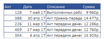

In this table, the Date and Amount column values ​​are formatted using the cell format. If you combine the values ​​as is (with the parameter disabled Use visible cell value), then you can get a not entirely correct result:


When merging, two columns were selected and in the group Unite item was selected each row of the range separately. To combine the first two columns (Act and Date), the separator “from” was used, for the 3rd and 4th (Description and Amount) - “to the amount: “. Paragraph Use visible cell value was disabled.
As you can see, the date doesn't look as expected. The amount too - rubles and the division of categories were lost.
But if you enable the item Use visible cell value, then the text in the merged cells will be exactly as it appears in the original cells: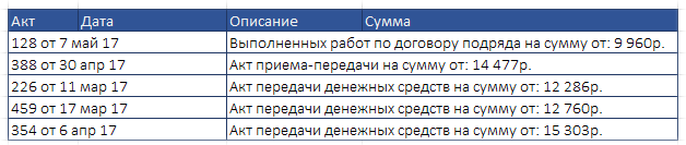

Hello, dear readers. Today we will talk about how you can combine two or more columns in an Excel table without losing data and values. You know that if you try to combine several columns into one, you will not succeed. Want to know how to do it right? Then let's get started.

The methods have been tested and work for any version of Excel. But as an example, I will be showing how to merge data without loss in Excel 2007.

For practice, I'll take a table where the cells are filled with cities, corresponding names and ages, and then merge them without losing content. Look at the screenshot.

Now, I’ll write a formula for connecting data from all cells of one row so that the contents are combined in it without losing the text.

First I will write it without spaces, otherwise Excel will throw an error. Any formula in Excel begins with the “=” sign, which means it will look like this =A2&B2&C2

As you can see, I ended up with a stuck together phrase. Agree, it’s not very nice. But now I can modify the formula to make the result readable. This is what the formula looks like now =A2&" "&B2&" "&C2. I can also place separation marks between them, for example a comma, and they will also be shown in the result.

Okay, I did one line. How will I spread the formula across other cells in the column? Now I won’t write it in every line. In my example there are only 4 of them, but what if there are a thousand of them? Of course I'll use a trick. Move the cursor to the edge of the cell so that it turns into a black square, and drag down to the end of the table. Look at the screenshot.

But that's not all. Although we have combined the columns, what do you think will happen if I change or delete the values ​​that I initially had? Then the result will change, because I used the formula, and its result is based on the data received. Something needs to be done about this.

Select the entire column with the merged content and copy (CTRL + C).

Then, in the adjacent empty column, in an empty cell, right-click and select “Paste Special” from the menu. And in the window that opens, check the “Values” box and click on “OK”.

Everything worked out for me. In each cell, I got the data from all cells and as text, which does not depend on the formula. Now I can delete all the columns I don’t need, or transfer the resulting data to a new table.

By the way, instead of the formula that I gave you above, you can use this: =CONCATENATE(A3; " "; B3; " "; C3). Two quotation marks with spaces are needed to ensure that there are spaces between the data when joining. But you can also put commas, pluses and other signs or even words in them. At your discretion.

Well friends, thanks for reading. I hope I helped you. Move on to other lessons, and don’t forget to subscribe, join the VKontakte group, comment, share on social networks, if you liked the lesson, let others get to know it.